文章作者:Tyan
博客:noahsnail.com | CSDN | 简书
声明:作者翻译论文仅为学习,如有侵权请联系作者删除博文,谢谢!
翻译论文汇总:https://github.com/SnailTyan/deep-learning-papers-translation
Deformable Convolutional Networks
Abstract
Convolutional neural networks (CNNs) are inherently limited to model geometric transformations due to the fixed geometric structures in their building modules. In this work, we introduce two new modules to enhance the transformation modeling capability of CNNs, namely, deformable convolution and deformable RoI pooling. Both are based on the idea of augmenting the spatial sampling locations in the modules with additional offsets and learning the offsets from the target tasks, without additional supervision. The new modules can readily replace their plain counterparts in existing CNNs and can be easily trained end-to-end by standard back-propagation, giving rise to deformable convolutional networks. Extensive experiments validate the performance of our approach. For the first time, we show that learning dense spatial transformation in deep CNNs is effective for sophisticated vision tasks such as object detection and semantic segmentation. The code is released at https://github.com/msracver/Deformable-ConvNets.
摘要
卷积神经网络(CNN)由于其构建模块固定的几何结构天然地局限于建模几何变换。在这项工作中,我们引入了两个新的模块来提高CNN的转换建模能力,即可变形卷积和可变形RoI池化。两者都基于这样的想法:增加模块中的空间采样位置以及额外的偏移量,并且从目标任务中学习偏移量,而不需要额外的监督。新模块可以很容易地替换现有CNN中的普通模块,并且可以通过标准的反向传播便易地进行端对端训练,从而产生可变形卷积网络。大量的实验验证了我们方法的性能。我们首次证明了在深度CNN中学习密集空间变换对于复杂的视觉任务(如目标检测和语义分割)是有效的。代码发布在https://github.com/msracver/Deformable-ConvNets。
1. Introduction
A key challenge in visual recognition is how to accommodate geometric variations or model geometric transformations in object scale, pose, viewpoint, and part deformation. In general, there are two ways. The first is to build the training datasets with sufficient desired variations. This is usually realized by augmenting the existing data samples, e.g., by affine transformation. Robust representations can be learned from the data, but usually at the cost of expensive training and complex model parameters. The second is to use transformation-invariant features and algorithms. This category subsumes many well known techniques, such as SIFT (scale invariant feature transform) [42] and sliding window based object detection paradigm.
1. 引言
视觉识别中的一个关键挑战是如何在目标尺度,姿态,视点和部件变形中适应几何变化或建模几何变换。一般来说,有两种方法。首先是建立具有足够期望变化的训练数据集。这通常通过增加现有的数据样本来实现,例如通过仿射变换。鲁棒的表示可以从数据中学习,但是通常以昂贵的训练和复杂的模型参数为代价。其次是使用变换不变的特征和算法。这一类包含了许多众所周知的技术,如SIFT(尺度不变特征变换)[42]和基于滑动窗口的目标检测范例。
There are two drawbacks in above ways. First, the geometric transformations are assumed fixed and known. Such prior knowledge is used to augment the data, and design the features and algorithms. This assumption prevents generalization to new tasks possessing unknown geometric transformations, which are not properly modeled. Second, hand-crafted design of invariant features and algorithms could be difficult or infeasible for overly complex transformations, even when they are known.
上述方法有两个缺点。首先,几何变换被假定是固定并且已知的。这样的先验知识被用来扩充数据,并设计特征和算法。这个假设阻止了对具有未知几何变换的新任务的泛化能力,这些新任务没有被正确地建模。其次,手工设计的不变特征和算法对于过于复杂的变换可能是困难的或不可行的,即使在已知复杂变化的情况下。
Recently, convolutional neural networks (CNNs) [35] have achieved significant success for visual recognition tasks, such as image classification [31], semantic segmentation [41], and object detection [16]. Nevertheless, they still share the above two drawbacks. Their capability of modeling geometric transformations mostly comes from the extensive data augmentation, the large model capacity, and some simple hand-crafted modules (e.g., max-pooling [1] for small translation-invariance).
最近,卷积神经网络(CNNs)[35]在图像分类[31],语义分割[41]和目标检测[16]等视觉识别任务中取得了显著的成功。不过,他们仍然有上述两个缺点。它们对几何变换建模的能力主要来自大量的数据增强,大的模型容量以及一些简单的手工设计模块(例如,对小的平移具有不变性的最大池化[1])。
In short, CNNs are inherently limited to model large, unknown transformations. The limitation originates from the fixed geometric structures of CNN modules: a convolution unit samples the input feature map at fixed locations; a pooling layer reduces the spatial resolution at a fixed ratio; a RoI (region-of-interest) pooling layer separates a RoI into fixed spatial bins, etc. There lacks internal mechanisms to handle the geometric transformations. This causes noticeable problems. For one example, the receptive field sizes of all activation units in the same CNN layer are the same. This is undesirable for high level CNN layers that encode the semantics over spatial locations. Because different locations may correspond to objects with different scales or deformation, adaptive determination of scales or receptive field sizes is desirable for visual recognition with fine localization, e.g., semantic segmentation using fully convolutional networks [41]. For another example, while object detection has seen significant and rapid progress [16, 52, 15, 47, 46, 40, 7] recently, all approaches still rely on the primitive bounding box based feature extraction. This is clearly sub-optimal, especially for non-rigid objects.
简而言之,CNN本质上局限于建模大型,未知的转换。该限制源于CNN模块的固定几何结构:卷积单元在固定位置对输入特征图进行采样;池化层以一个固定的比例降低空间分辨率;一个RoI(感兴趣区域)池化层把RoI分成固定的空间组块等等。缺乏处理几何变换的内部机制。这会导致明显的问题。举一个例子,同一CNN层中所有激活单元的感受野大小是相同的。对于在空间位置上编码语义的高级CNN层来说,这是不可取的。由于不同的位置可能对应不同尺度或形变的目标,所以对于具有精细定位的视觉识别来说,例如使用全卷积网络的语义分割[41],尺度或感受野大小的自适应确定是理想的情况。又如,尽管最近目标检测已经取得了显著而迅速的进展[16,52,15,47,46,40,7],但所有方法仍然依赖于基于特征提取的粗糙边界框。这显然是次优的,特别是对于非刚性目标。
In this work, we introduce two new modules that greatly enhance CNNs’ capability of modeling geometric transformations. The first is deformable convolution. It adds 2D offsets to the regular grid sampling locations in the standard convolution. It enables free form deformation of the sampling grid. It is illustrated in Figure 1. The offsets are learned from the preceding feature maps, via additional convolutional layers. Thus, the deformation is conditioned on the input features in a local, dense, and adaptive manner.
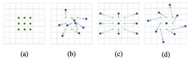
Figure 1: Illustration of the sampling locations in 3 × 3 standard and deformable convolutions. (a) regular sampling grid (green points) of standard convolution. (b) deformed sampling locations (dark blue points) with augmented offsets (light blue arrows) in deformable convolution. (c)(d) are special cases of (b), showing that the deformable convolution generalizes various transformations for scale, (anisotropic) aspect ratio and rotation.
在这项工作中,我们引入了两个新的模块,大大提高了CNN建模几何变换的能力。首先是可变形卷积。它将2D偏移添加到标准卷积中的常规网格采样位置上。它可以使采样网格自由形变。如图1所示。偏移量通过附加的卷积层从前面的特征图中学习。因此,变形以局部的,密集的和自适应的方式受到输入特征的限制。
图1:3×3标准卷积和可变形卷积中采样位置的示意图。(a)标准卷积的定期采样网格(绿点)。(b)变形的采样位置(深蓝色点)和可变形卷积中增大的偏移量(浅蓝色箭头)。(c)(d)是(b)的特例,表明可变形卷积泛化到了各种尺度(各向异性)、长宽比和旋转的变换。
The second is deformable RoI pooling. It adds an offset to each bin position in the regular bin partition of the previous RoI pooling [15, 7]. Similarly, the offsets are learned from the preceding feature maps and the RoIs, enabling adaptive part localization for objects with different shapes.
第二个是可变形的RoI池化。它为前面的RoI池化的常规bin分区中的每个bin位置添加一个偏移量[15,7]。类似地,从前面的特征映射和RoI中学习偏移量,使得具有不同形状的目标能够自适应的进行部件定位。
Both modules are light weight. They add small amount of parameters and computation for the offset learning. They can readily replace their plain counterparts in deep CNNs and can be easily trained end-to-end with standard back-propagation. The resulting CNNs are called deformable convolutional networks, or deformable ConvNets.
两个模块都轻量的。它们为偏移学习增加了少量的参数和计算。他们可以很容易地取代深层CNN中简单的对应部分,并且可以很容易地通过标准的反向传播进行端对端的训练。所得到的CNN被称为可变形卷积网络,或可变形ConvNets。
Our approach shares similar high level spirit with spatial transform networks [26] and deformable part models [11]. They all have internal transformation parameters and learn such parameters purely from data. A key difference in deformable ConvNets is that they deal with dense spatial transformations in a simple, efficient, deep and end-to-end manner. In Section 3.1, we discuss in details the relation of our work to previous works and analyze the superiority of deformable ConvNets.
我们的方法与空间变换网络[26]和可变形部件模型[11]具有类似的高层精神。它们都有内部的转换参数,纯粹从数据中学习这些参数。可变形ConvNets的一个关键区别在于它们以简单,高效,深入和端到端的方式处理密集的空间变换。在3.1节中,我们详细讨论了我们的工作与以前的工作的关系,并分析了可变形ConvNets的优越性。
2. Deformable Convolutional Networks
The feature maps and convolution in CNNs are 3D. Both deformable convolution and RoI pooling modules operate on the 2D spatial domain. The operation remains the same across the channel dimension. Without loss of generality, the modules are described in 2D here for notation clarity. Extension to 3D is straightforward.
2. 可变形卷积网络
CNN中的特征映射和卷积是3D的。可变形卷积和RoI池化模块都在2D空间域上运行。在整个通道维度上的操作保持不变。在不丧失普遍性的情况下,为了符号清晰,这些模块在2D中描述。扩展到3D很简单。
2.1. Deformable Convolution
The 2D convolution consists of two steps: 1) sampling using a regular grid $\mathcal{R}$ over the input feature map $\mathbf{x}$; 2) summation of sampled values weighted by $\mathbf{w}$. The grid $\mathcal{R}$ defines the receptive field size and dilation. For example, $$\mathcal{R}=\lbrace (-1, -1), (-1, 0), \ldots, (0,1), (1, 1)\rbrace$$ defines a $3 \times 3$ kernel with dilation $1$.
2.1. 可变形卷积
2D卷积包含两步:1)用规则的网格$\mathcal{R}$在输入特征映射$\mathbf{x}$上采样;2)对$\mathbf{w}$加权的采样值求和。网格$\mathcal{R}$定义了感受野的大小和扩张。例如,$$\mathcal{R}=\lbrace (-1, -1), (-1, 0), \ldots, (0,1), (1, 1)\rbrace$$定义了一个扩张大小为$1$的$3 \times 3$卷积核。
For each location $\mathbf{p}_0$ on the output feature map $\mathbf{y}$, we have $$\mathbf{y}(\mathbf{p}_0)=\sum_{\mathbf{p}_n\in\mathcal{R}}\mathbf{w}(\mathbf{p}_n)\cdot \mathbf{x}(\mathbf{p}_0+\mathbf{p}_n) \tag{1}$$ where $\mathbf{p}_n$ enumerates the locations in $\mathcal{R}$.
对于输出特征映射$\mathbf{y}$上的每个位置$\mathbf{p}_0$,我们有$$\mathbf{y}(\mathbf{p}_0)=\sum_{\mathbf{p}_n\in\mathcal{R}}\mathbf{w}(\mathbf{p}_n)\cdot \mathbf{x}(\mathbf{p}_0+\mathbf{p}_n) \tag{1}$$其中$\mathbf{p}_n$枚举了$\mathcal{R}$中的位置。
In deformable convolution, the regular grid $\mathcal{R}$ is augmented with offsets $\lbrace \Delta \mathbf{p}_n|n=1,…,N\rbrace$, where $N=|\mathcal{R}|$. Eq.(1) becomes $$\mathbf{y}(\mathbf{p}_0)=\sum_{\mathbf{p}_n\in\mathcal{R}}\mathbf{w}(\mathbf{p}_n)\cdot \mathbf{x}(\mathbf{p}_0+\mathbf{p}_n+\Delta \mathbf{p}_n).\tag{2}$$
在可变形卷积中,规则的网格$\mathcal{R}$通过偏移$\lbrace \Delta \mathbf{p}_n|n=1,…,N\rbrace$增大,其中$N=|\mathcal{R}|$。方程(1)变为$$\mathbf{y}(\mathbf{p}_0)=\sum_{\mathbf{p}_n\in\mathcal{R}}\mathbf{w}(\mathbf{p}_n)\cdot \mathbf{x}(\mathbf{p}_0+\mathbf{p}_n+\Delta \mathbf{p}_n).\tag{2}$$
Now, the sampling is on the irregular and offset locations $\mathbf{p}_n + \Delta \mathbf{p}_n$. As the offset $\Delta \mathbf{p}_n$ is typically fractional, Eq.(2) is implemented via bilinear interpolation as $$\mathbf{x}(\mathbf{p})=\sum_\mathbf{q} G(\mathbf{q},\mathbf{p})\cdot \mathbf{x}(\mathbf{q}), \tag{3} $$ where $\mathbf{p}$ denotes an arbitrary (fractional) location ($\mathbf{p}=\mathbf{p}_0+\mathbf{p}_n+\Delta \mathbf{p}_n$ for Eq.(2)), $\mathbf{q}$ enumerates all integral spatial locations in the feature map $\mathbf{x}$, and $G(\cdot,\cdot)$ is the bilinear interpolation kernel. Note that $G$ is two dimensional. It is separated into two one dimensional kernels as $$ G(\mathbf{q},\mathbf{p})=g(q_x,p_x)\cdot g(q_y,p_y), \tag{4}$$ where $g(a,b)=max(0,1-|a-b|)$. Eq.(3) is fast to compute as $G(\mathbf{q},\mathbf{p})$ is non-zero only for a few $\mathbf{q}$s.
现在,采样是在不规则且有偏移的位置$\mathbf{p}_n + \Delta \mathbf{p}_n$上。由于偏移$\Delta \mathbf{p}_n$通常是小数,方程(2)可以通过双线性插值实现$$\mathbf{x}(\mathbf{p})=\sum_\mathbf{q} G(\mathbf{q},\mathbf{p})\cdot \mathbf{x}(\mathbf{q}), \tag{3} $$其中$\mathbf{p}$表示任意(小数)位置(公式(2)中$\mathbf{p}=\mathbf{p}_0+\mathbf{p}_n+\Delta \mathbf{p}_n$),$\mathbf{q}$枚举了特征映射$\mathbf{x}$中所有整体空间位置,$G(\cdot,\cdot)$是双线性插值的核。注意$G$是二维的。它被分为两个一维核$$ G(\mathbf{q},\mathbf{p})=g(q_x,p_x)\cdot g(q_y,p_y), \tag{4}$$其中$g(a,b)=max(0,1-|a-b|)$。方程(3)可以快速计算因为$G(\mathbf{q},\mathbf{p})$仅对于一些$\mathbf{q}$是非零的。
As illustrated in Figure 2, the offsets are obtained by applying a convolutional layer over the same input feature map. The convolution kernel is of the same spatial resolution and dilation as those of the current convolutional layer (e.g., also $3\times 3$ with dilation 1 in Figure 2. The output offset fields have the same spatial resolution with the input feature map. The channel dimension $2N$ corresponds to $N$ 2D offsets. During training, both the convolutional kernels for generating the output features and the offsets are learned simultaneously. To learn the offsets, the gradients are back-propagated through the bilinear operations in Eq.(3) and Eq.(4). It is detailed in appendix A.
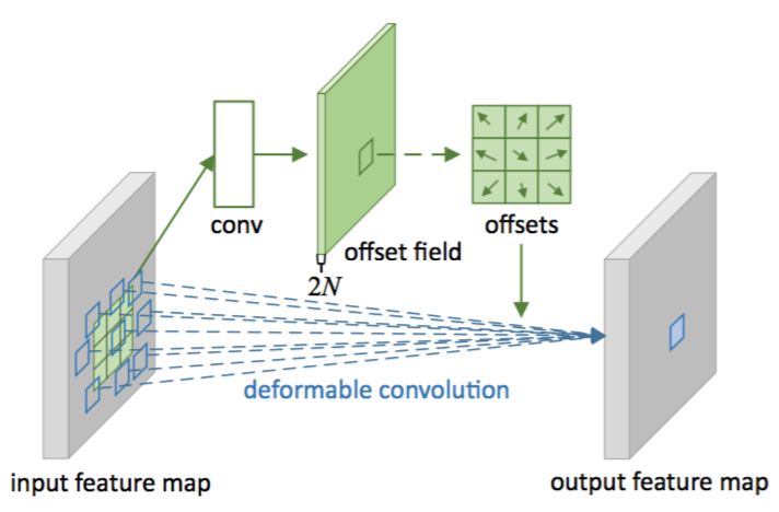
Figure 2: Illustration of 3 × 3 deformable convolution.
如图2所示,通过在相同的输入特征映射上应用卷积层来获得偏移。卷积核具有与当前卷积层相同的空间分辨率和扩张(例如,在图2中也具有扩张为1的$3\times 3$)。输出偏移域与输入特征映射具有相同的空间分辨率。通道维度$2N$(注释:偏移的通道维度,包括$x$方向的通道维度和$y$方向的通道维度)对应于$N$个2D偏移量。在训练过程中,同时学习用于生成输出特征的卷积核和偏移量。为了学习偏移量,梯度通过方程(3)和(4)中的双线性运算进行反向传播。详见附录A。
图2:3×3可变形卷积的说明。
2.2. Deformable RoI Pooling
RoI pooling is used in all region proposal based object detection methods [16, 15, 47, 7]. It converts an input rectangular region of arbitrary size into fixed size features.
2.2. 可变形RoI池化
在所有基于区域提出的目标检测方法中都使用了RoI池化[16,15,47,7]。它将任意大小的输入矩形区域转换为固定大小的特征。
RoI Pooling [15] Given the input feature map $\mathbf{x}$ and a RoI of size $w\times h$ and top-left corner $\mathbf{p}_0$, RoI pooling divides the RoI into $k\times k$ ($k$ is a free parameter) bins and outputs a $k\times k$ feature map $\mathbf{y}$. For $(i,j)$-th bin ($0\le i,j < k$), we have $$\mathbf{y}(i,j)=\sum_{\mathbf{p}\in bin(i,j)} \mathbf{x}(\mathbf{p}_0+\mathbf{p})/n_{ij},\tag{5}$$ where $n_{ij}$ is the number of pixels in the bin. The $(i,j)$-th bin spans $\lfloor i \frac{w}{k} \rfloor \le p_x < \lceil (i+1)\frac{w}{k}\rceil$ and $\lfloor j \frac{h}{k}\rfloor \le p_y < \lceil (j+1)\frac{h}{k} \rceil$.
RoI池化[15]。给定输入特征映射$\mathbf{x}$、RoI的大小$w\times h$和左上角$\mathbf{p}_0$,RoI池化将ROI分到$k\times k$($k$是一个自由参数)个组块(bin)中,并输出$k\times k$的特征映射$\mathbf{y}$。对于第$(i,j)$个组块($0\le i,j < k$),我们有$$\mathbf{y}(i,j)=\sum_{\mathbf{p}\in bin(i,j)} \mathbf{x}(\mathbf{p}_0+\mathbf{p})/n_{ij},\tag{5}$$其中$n_{ij}$是组块中的像素数量。第$(i,j)$个组块的跨度为$\lfloor i \frac{w}{k} \rfloor \le p_x < \lceil (i+1)\frac{w}{k}\rceil$和$\lfloor j \frac{h}{k}\rfloor \le p_y < \lceil (j+1)\frac{h}{k} \rceil$。
Similarly as in Eq.(2), in deformable RoI pooling, offsets ${\Delta \mathbf{p}_{ij}|0\le i,j < k}$ are added to the spatial binning positions. Eq.(5) becomes $$\mathbf{y}(i,j)=\sum_{\mathbf{p}\in bin(i,j)} \mathbf{x}(\mathbf{p}_0+\mathbf{p}+\Delta \mathbf{p}_{ij})/n_{ij}. \tag{6}$$ Typically, $\Delta \mathbf{p}_{ij}$ is fractional. Eq.(6) is implemented by bilinear interpolation via Eq.(3) and (4).
类似于方程(2),在可变形RoI池化中,将偏移${\Delta \mathbf{p}_{ij}|0\le i,j < k}$加到空间组块的位置上。方程(5)变为$$\mathbf{y}(i,j)=\sum_{\mathbf{p}\in bin(i,j)} \mathbf{x}(\mathbf{p}_0+\mathbf{p}+\Delta \mathbf{p}_{ij})/n_{ij}. \tag{6}$$通常,$\Delta \mathbf{p}_{ij}$是小数。方程(6)通过双线性插值方程(3)和(4)来实现。
Figure 3 illustrates how to obtain the offsets. Firstly, RoI pooling (Eq.(5)) generates the pooled feature maps. From the maps, a fc layer generates the normalized offsets $\Delta \widehat{\mathbf{p}}_{ij}$, which are then transformed to the offsets $\Delta \mathbf{p}_{ij}$ in Eq.(6) by element-wise product with the RoI’s width and height, as $\Delta \mathbf{p}_{ij} = \gamma \cdot \Delta \widehat{\mathbf{p}}_{ij} \circ (w, h)$. Here $\gamma$ is a pre-defined scalar to modulate the magnitude of the offsets. It is empirically set to $\gamma=0.1$. The offset normalization is necessary to make the offset learning invariant to RoI size. The fc layer is learned by back-propagation, as detailed in appendix A.
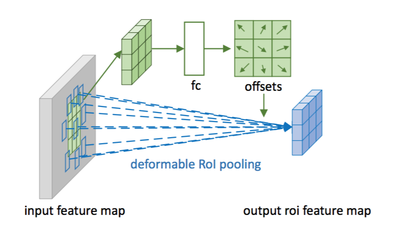
Figure 3: Illustration of 3 × 3 deformable RoI pooling.
图3说明了如何获得偏移量。首先,RoI池化(方程(5))生成池化后的特征映射。从特征映射中,一个fc层产生归一化偏移量$\Delta \widehat{\mathbf{p}}_{ij}$,然后通过与RoI的宽和高进行逐元素的相乘将其转换为方程(6)中的偏移量$\Delta \mathbf{p}_{ij}$,如:$\Delta \mathbf{p}_{ij} = \gamma \cdot \Delta \widehat{\mathbf{p}}_{ij} \circ (w, h)$。这里$\gamma$是一个预定义的标量来调节偏移的大小。它经验地设定为$\gamma=0.1$。为了使偏移学习对RoI大小具有不变性,偏移归一化是必要的。fc层是通过反向传播学习,详见附录A。
图3:阐述3×3的可变形RoI池化。
Position-Sensitive (PS) RoI Pooling [7] It is fully convolutional and different from RoI pooling. Through a conv layer, all the input feature maps are firstly converted to $k^2$ score maps for each object class (totally $C+1$ for $C$ object classes), as illustrated in the bottom branch in Figure 4. Without need to distinguish between classes, such score maps are denoted as $\lbrace \mathbf{x}_{i,j}\rbrace$ where $(i,j)$ enumerates all bins. Pooling is performed on these score maps. The output value for $(i,j)$-th bin is obtained by summation from one score map $\mathbf{x}_{i,j}$ corresponding to that bin. In short, the difference from RoI pooling in Eq.(5) is that a general feature map $\mathbf{x}$ is replaced by a specific positive-sensitive score map $\mathbf{x}_{i,j}$.
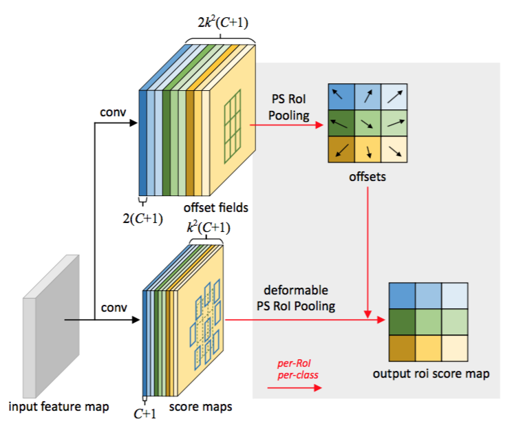
Figure 4: Illustration of 3 × 3 deformable PS RoI pooling.
位置敏感(PS)的RoI池化[7]。它是全卷积的,不同于RoI池化。通过一个卷积层,所有的输入特征映射首先被转换为每个目标类的$k^2$个分数映射(对于$C$个目标类,总共$C+1$个),如图4的底部分支所示。不需要区分类,这样的分数映射被表示为$\lbrace \mathbf{x}_{i,j}\rbrace$,其中$(i,j)$枚举所有的组块。池化是在这些分数映射上进行的。第$(i,j)$个组块的输出值是通过对分数映射$\mathbf{x}_{i,j}$对应的组块求和得到的。简而言之,与方程(5)中RoI池化的区别在于,通用特征映射$\mathbf{x}$被特定的位置敏感的分数映射$\mathbf{x}_{i,j}$所取代。
图4:阐述3×3的可变形PS RoI池化。
In deformable PS RoI pooling, the only change in Eq.(6) is that $\mathbf{x}$ is also modified to $\mathbf{x}_{i,j}$. However, the offset learning is different. It follows the fully convolutional spirit in [7], as illustrated in Figure 4. In the top branch, a conv layer generates the full spatial resolution offset fields. For each RoI (also for each class), PS RoI pooling is applied on such fields to obtain normalized offsets $\Delta \widehat{\mathbf{p}}_{ij}$, which are then transformed to the real offsets $\Delta \mathbf{p}_{ij}$ in the same way as in deformable RoI pooling described above.
在可变形PS RoI池化中,方程(6)中唯一的变化是$\mathbf{x}$也被修改为$\mathbf{x}_{i,j}$。但是,偏移学习是不同的。它遵循[7]中的“全卷积”精神,如图4所示。在顶部分支中,一个卷积层生成完整空间分辨率的偏移量字段。对于每个RoI(也对于每个类),在这些字段上应用PS RoI池化以获得归一化偏移量$\Delta \widehat{\mathbf{p}}_{ij}$,然后以上面可变形RoI池化中描述的相同方式将其转换为实数偏移量$\Delta \mathbf{p}_{ij}$。
2.3. Deformable ConvNets
Both deformable convolution and RoI pooling modules have the same input and output as their plain versions. Hence, they can readily replace their plain counterparts in existing CNNs. In the training, these added conv and fc layers for offset learning are initialized with zero weights. Their learning rates are set to $\beta$ times ($\beta = 1$ by default, and $\beta = 0.01$ for the fc layer in Faster R-CNN) of the learning rate for the existing layers. They are trained via back propagation through the bilinear interpolation operations in Eq.(3) and Eq.(4). The resulting CNNs are called deformable ConvNets.
2.3. 可变形卷积网络
可变形卷积和RoI池化模块都具有与普通版本相同的输入和输出。因此,它们可以很容易地取代现有CNN中的普通版本。在训练中,这些添加的用于偏移学习的conv和fc层的权重被初始化为零。它们的学习率设置为现有层学习速率的$\beta$倍(默认$\beta=1$,Faster R-CNN中的fc层为$\beta=0.01$)。它们通过方程(3)和方程(4)中双线性插值运算的反向传播进行训练。由此产生的CNN称为可变形ConvNets。
To integrate deformable ConvNets with the state-of-the-art CNN architectures, we note that these architectures consist of two stages. First, a deep fully convolutional network generates feature maps over the whole input image. Second, a shallow task specific network generates results from the feature maps. We elaborate the two steps below.
为了将可变形的ConvNets与最先进的CNN架构集成,我们注意到这些架构由两个阶段组成。首先,深度全卷积网络在整个输入图像上生成特征映射。其次,浅层任务专用网络从特征映射上生成结果。我们详细说明下面两个步骤。
Deformable Convolution for Feature Extraction We adopt two state-of-the-art architectures for feature extraction: ResNet-101 [22] and a modifed version of Inception-ResNet [51]. Both are pre-trained on ImageNet [8] classification dataset.
特征提取的可变形卷积。我们采用两种最先进的架构进行特征提取:ResNet-101[22]和Inception-ResNet[51]的修改版本。两者都在ImageNet[8]分类数据集上进行预训练。
The original Inception-ResNet is designed for image recognition. It has a feature misalignment issue and problematic for dense prediction tasks. It is modified to fix the alignment problem [20]. The modified version is dubbed as “Aligned-Inception-ResNet” and is detailed in appendix B.
最初的Inception-ResNet是为图像识别而设计的。它有一个特征不对齐的问题,对于密集的预测任务是有问题的。它被修改来解决对齐问题[20]。修改后的版本被称为“Aligned-Inception-ResNet”,详见附录B.
Both models consist of several convolutional blocks, an average pooling and a 1000-way fc layer for ImageNet classification. The average pooling and the fc layers are removed. A randomly initialized 1 × 1 convolution is added at last to reduce the channel dimension to 1024. As in common practice [4, 7], the effective stride in the last convolutional block is reduced from 32 pixels to 16 pixels to increase the feature map resolution. Specifically, at the beginning of the last block, stride is changed from 2 to 1 (“conv5” for both ResNet-101 and Aligned-Inception-ResNet). To compensate, the dilation of all the convolution filters in this block (with kernel size > 1) is changed from 1 to 2.
两种模型都由几个卷积块组成,平均池化和用于ImageNet分类的1000类全连接层。平均池化和全连接层被移除。最后加入随机初始化的1×1卷积,以将通道维数减少到1024。与通常的做法[4,7]一样,最后一个卷积块的有效步长从32个像素减少到16个像素,以增加特征映射的分辨率。具体来说,在最后一个块的开始,步长从2变为1(ResNet-101和Aligned-Inception-ResNet的“conv5”)。为了进行补偿,将该块(核大小>1)中的所有卷积滤波器的扩张从1改变为2。
Optionally, deformable convolution is applied to the last few convolutional layers (with kernel size > 1). We experimented with different numbers of such layers and found 3 as a good trade-off for different tasks, as reported in Table 1.
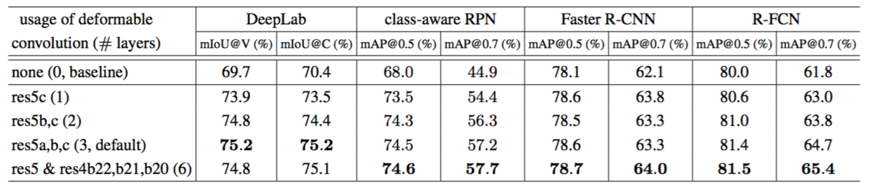
Table 1: Results of using deformable convolution in the last 1, 2, 3, and 6 convolutional layers (of 3 × 3 filter) in ResNet-101 feature extraction network. For class-aware RPN, Faster R-CNN, and R-FCN, we report result on VOC 2007 test.
可选地,可变形卷积应用于最后的几个卷积层(核大小>1)。我们尝试了不同数量的这样的层,发现3是不同任务的一个很好的权衡,如表1所示。
表1:在ResNet-101特征提取网络中的最后1个,2个,3个和6个卷积层上(3×3滤波器)应用可变形卷积的结果。对于class-aware RPN,Faster R-CNN和R-FCN,我们报告了在VOC 2007测试集上的结果。
Segmentation and Detection Networks A task specific network is built upon the output feature maps from the feature extraction network mentioned above.
分割和检测网络。根据上述特征提取网络的输出特征映射构建特定任务的网络。
In the below, $C$ denotes the number of object classes.
在下面,$C$表示目标类别的数量。
DeepLab [5] is a state-of-the-art method for semantic segmentation. It adds a 1 × 1 convolutional layer over the feature maps to generates (C + 1) maps that represent the per-pixel classification scores. A following softmax layer then outputs the per-pixel probabilities.
DeepLab[5]是最先进的语义分割方法。它在特征映射上添加1×1卷积层以生成表示每个像素分类分数的(C+1)个映射。然后随后的softmax层输出每个像素的概率。
Category-Aware RPN is almost the same as the region proposal network in [47], except that the 2-class (object or not) convolutional classifier is replaced by a (C + 1)-class convolutional classifier. It can be considered as a simplified version of SSD [40].
除了用(C+1)类卷积分类器代替2类(目标或非目标)卷积分类器外,Category-Aware RPN与[47]中的区域提出网络几乎是相同的。它可以被认为是SSD的简化版本[40]。
Faster R-CNN [47] is the state-of-the-art detector. In our implementation, the RPN branch is added on the top of the conv4 block, following [47]. In the previous practice [22, 24], the RoI pooling layer is inserted between the conv4 and the conv5 blocks in ResNet-101, leaving 10 layers for each RoI. This design achieves good accuracy but has high per-RoI computation. Instead, we adopt a simplified design as in [38]. The RoI pooling layer is added at last. On top of the pooled RoI features, two fc layers of dimension 1024 are added, followed by the bounding box regression and the classification branches. Although such simplification (from 10 layer conv5 block to 2 fc layers) would slightly decrease the accuracy, it still makes a strong enough baseline and is not a concern in this work.
Faster R-CNN[47]是最先进的检测器。在我们的实现中,RPN分支被添加在conv4块的顶部,遵循[47]。在以前的实践中[22,24],在ResNet-101的conv4和conv5块之间插入了RoI池化层,每个RoI留下了10层。这个设计实现了很好的精确度,但是具有很高的每个RoI计算。相反,我们采用[38]中的简化设计。RoI池化层在最后添加。在池化的RoI特征之上,添加了两个1024维的全连接层,接着是边界框回归和分类分支。虽然这样的简化(从10层conv5块到2个全连接层)会稍微降低精确度,但它仍然具有足够强的基准,在这项工作中不再关心。
Optionally, the RoI pooling layer can be changed to deformable RoI pooling.
可选地,可以将RoI池化层更改为可变形的RoI池化。
R-FCN [7] is another state-of-the-art detector. It has negligible per-RoI computation cost. We follow the original implementation. Optionally, its RoI pooling layer can be changed to deformable position-sensitive RoI pooling.
R-FCN[7]是另一种最先进的检测器。它的每个RoI计算成本可以忽略不计。我们遵循原来的实现。可选地,其RoI池化层可以改变为可变形的位置敏感的RoI池化。
3. Understanding Deformable ConvNets
This work is built on the idea of augmenting the spatial sampling locations in convolution and RoI pooling with additional offsets and learning the offsets from target tasks.
3. 理解可变形卷积网络
这项工作以用额外的偏移量在卷积和RoI池中增加空间采样位置,并从目标任务中学习偏移量的想法为基础。
When the deformable convolution are stacked, the effect of composited deformation is profound. This is exemplified in Figure 5. The receptive field and the sampling locations in the standard convolution are fixed all over the top feature map (left). They are adaptively adjusted according to the objects’ scale and shape in deformable convolution (right). More examples are shown in Figure 6. Table 2 provides quantitative evidence of such adaptive deformation.
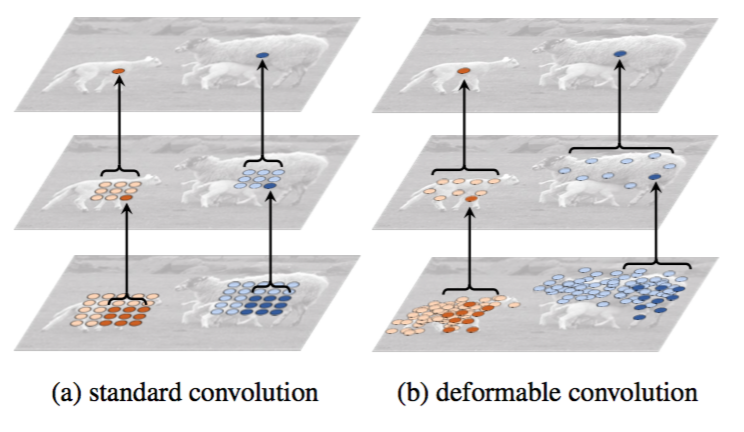
Figure 5: Illustration of the fixed receptive field in standard convolution (a) and the adaptive receptive field in deformable convolution (b), using two layers. Top: two activation units on the top feature map, on two objects of different scales and shapes. The activation is from a 3 × 3 filter. Middle: the sampling locations of the 3 × 3 filter on the preceding feature map. Another two activation units are highlighted. Bottom: the sampling locations of two levels of 3 × 3 filters on the preceding feature map. Two sets of locations are highlighted, corresponding to the highlighted units above.
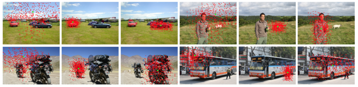
Figure 6: Each image triplet shows the sampling locations ($9^3 = 729$ red points in each image) in three levels of 3 × 3 deformable filters (see Figure 5 as a reference) for three activation units (green points) on the background (left), a small object (middle), and a large object (right), respectively.
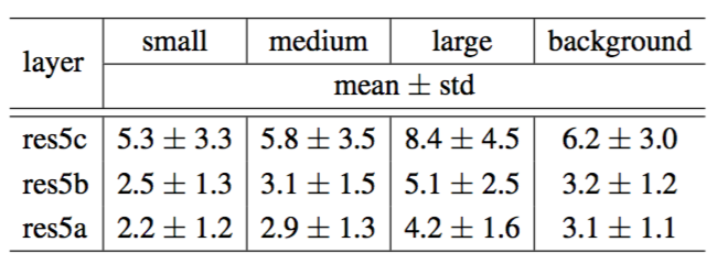
Table 2: Statistics of effective dilation values of deformable convolutional filters on three layers and four categories. Similar as in COCO [39], we divide the objects into three categories equally according to the bounding box area. Small: area < $96^2$ pixels; medium: $96^2$ < area < $224^2$; large: area > $224^2$ pixels.
当可变形卷积叠加时,复合变形的影响是深远的。这在图5中举例说明。标准卷积中的感受野和采样位置在顶部特征映射上是固定的(左)。它们在可变形卷积中(右)根据目标的尺寸和形状进行自适应调整。图6中显示了更多的例子。表2提供了这种自适应变形的量化证据。
图5:标准卷积(a)中的固定感受野和可变形卷积(b)中的自适应感受野的图示,使用两层。顶部:顶部特征映射上的两个激活单元,在两个不同尺度和形状的目标上。激活来自3×3滤波器。中间:前一个特征映射上3×3滤波器的采样位置。另外两个激活单元突出显示。底部:前一个特征映射上两个3×3滤波器级别的采样位置。突出显示两组位置,对应于上面突出显示的单元。
图6:每个图像三元组在三级3×3可变形滤波器(参见图5作为参考)中显示了三个激活单元(绿色点)分别在背景(左)、小目标(中)和大目标(右)上的采样位置(每张图像中的$9^3 = 729$个红色点)。
表2:可变形卷积滤波器在三个卷积层和四个类别上的有效扩张值的统计。与在COCO[39]中类似,我们根据边界框区域将目标平均分为三类。小:面积<$96^2$个像素;中等:$96^2$<面积<$224^2$; 大:面积>$224^2$。
The effect of deformable RoI pooling is similar, as illustrated in Figure 7. The regularity of the grid structure in standard RoI pooling no longer holds. Instead, parts deviate from the RoI bins and move onto the nearby object foreground regions. The localization capability is enhanced, especially for non-rigid objects.
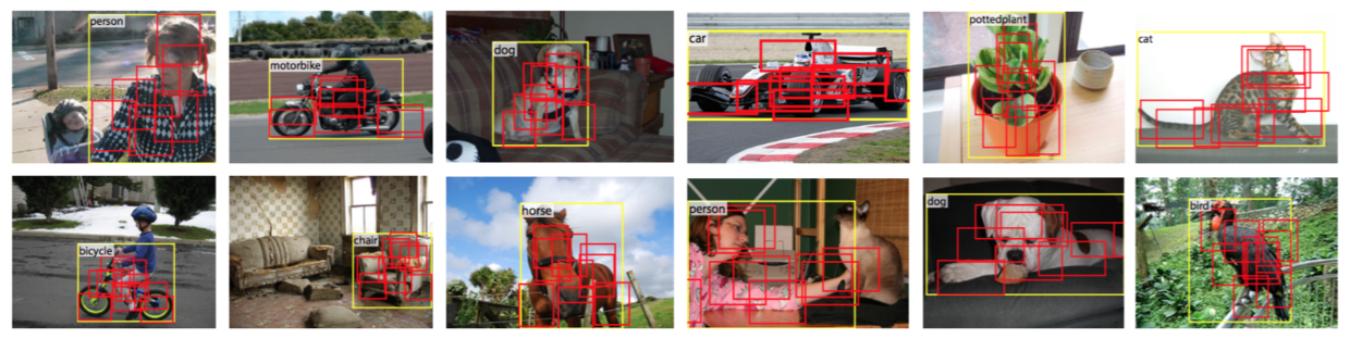
Figure 7: Illustration of offset parts in deformable (positive sensitive) RoI pooling in R-FCN [7] and 3 × 3 bins (red) for an input RoI (yellow). Note how the parts are offset to cover the non-rigid objects.
可变形RoI池化的效果是类似的,如图7所示。标准RoI池化中网格结构的规律不再成立。相反,部分偏离RoI组块并移动到附近的目标前景区域。定位能力得到增强,特别是对于非刚性物体。
图7:R-FCN[7]中可变形(正敏感)RoI池化的偏移部分的示意图和输入RoI(黄色)的3x3个组块(红色)。请注意部件如何偏移以覆盖非刚性物体。
3.1. In Context of Related Works
Our work is related to previous works in different aspects. We discuss the relations and differences in details.
3.1. 相关工作的背景
我们的工作与以前的工作在不同的方面有联系。我们详细讨论联系和差异。
Spatial Transform Networks (STN) [26] It is the first work to learn spatial transformation from data in a deep learning framework. It warps the feature map via a global parametric transformation such as affine transformation. Such warping is expensive and learning the transformation parameters is known difficult. STN has shown successes in small scale image classification problems. The inverse STN method [37] replaces the expensive feature warping by efficient transformation parameter propagation.
空间变换网络(STN)[26]。这是在深度学习框架下从数据中学习空间变换的第一个工作。它通过全局参数变换扭曲特征映射,例如仿射变换。这种扭曲是昂贵的,学习变换参数是困难的。STN在小规模图像分类问题上取得了成功。反STN方法[37]通过有效的变换参数传播来代替昂贵的特征扭曲。
The offset learning in deformable convolution can be considered as an extremely light-weight spatial transformer in STN [26]. However, deformable convolution does not adopt a global parametric transformation and feature warping. Instead, it samples the feature map in a local and dense manner. To generate new feature maps, it has a weighted summation step, which is absent in STN.
可变形卷积中的偏移学习可以被认为是STN中极轻的空间变换器[26]。然而,可变形卷积不采用全局参数变换和特征扭曲。相反,它以局部密集的方式对特征映射进行采样。为了生成新的特征映射,它有加权求和步骤,STN中不存在。
Deformable convolution is easy to integrate into any CNN architectures. Its training is easy. It is shown effective for complex vision tasks that require dense (e.g., semantic segmentation) or semi-dense (e.g., object detection) predictions. These tasks are difficult (if not infeasible) for STN [26, 37].
可变形卷积很容易集成到任何CNN架构中。它的训练很简单。对于要求密集(例如语义分割)或半密集(例如目标检测)预测的复杂视觉任务来说,它是有效的。这些任务对于STN来说是困难的(如果不是不可行的话)[26,37]。
Active Convolution [27] This work is contemporary. It also augments the sampling locations in the convolution with offsets and learns the offsets via back-propagation end-to-end. It is shown effective on image classification tasks.
主动卷积[27]。这项工作是当代的。它还通过偏移来增加卷积中的采样位置,并通过端到端的反向传播学习偏移量。它对于图像分类任务是有效的。
Two crucial differences from deformable convolution make this work less general and adaptive. First, it shares the offsets all over the different spatial locations. Second, the offsets are static model parameters that are learnt per task or per training. In contrast, the offsets in deformable convolution are dynamic model outputs that vary per image location. They model the dense spatial transformations in the images and are effective for (semi-)dense prediction tasks such as object detection and semantic segmentation.
与可变形卷积的两个关键区别使得这个工作不那么一般和适应。首先,它在所有不同的空间位置上共享偏移量。其次,偏移量是每个任务或每次训练都要学习的静态模型参数。相反,可变形卷积中的偏移是每个图像位置变化的动态模型输出。他们对图像中的密集空间变换进行建模,对于(半)密集的预测任务(如目标检测和语义分割)是有效的。
Effective Receptive Field [43] It finds that not all pixels in a receptive field contribute equally to an output response. The pixels near the center have much larger impact. The effective receptive field only occupies a small fraction of the theoretical receptive field and has a Gaussian distribution. Although the theoretical receptive field size increases linearly with the number of convolutional layers, a surprising result is that, the effective receptive field size increases linearly with the square root of the number, therefore, at a much slower rate than what we would expect.
有效的感受野[43]。它发现,并不是感受野中的所有像素都贡献平等的输出响应。中心附近的像素影响更大。有效感受野只占据理论感受野的一小部分,并具有高斯分布。虽然理论上的感受野大小随卷积层数量线性增加,但令人惊讶的结果是,有效感受野大小随着数量的平方根线性增加,因此,感受野大小以比我们期待的更低的速率增加。
This finding indicates that even the top layer’s unit in deep CNNs may not have large enough receptive field. This partially explains why atrous convolution [23] is widely used in vision tasks (see below). It indicates the needs of adaptive receptive field learning.
这一发现表明,即使是深层CNN的顶层单元也可能没有足够大的感受野。这部分解释了为什么空洞卷积[23]被广泛用于视觉任务(见下文)。它表明了自适应感受野学习的必要。
Deformable convolution is capable of learning receptive fields adaptively, as shown in Figure 5, 6 and Table 2.
可变形卷积能够自适应地学习感受野,如图5,6和表2所示。
Atrous convolution [23] It increases a normal filter’s stride to be larger than 1 and keeps the original weights at sparsified sampling locations. This increases the receptive field size and retains the same complexity in parameters and computation. It has been widely used for semantic segmentation [41, 5, 54] (also called dilated convolution in [54]), object detection [7], and image classification [55].
空洞卷积[23]。它将正常滤波器的步长增加到大于1,并保持稀疏采样位置的原始权重。这增加了感受野的大小,并保持了相同的参数和计算复杂性。它已被广泛用于语义分割[41,5,54](在[54]中也称扩张卷积),目标检测[7]和图像分类[55]。
Deformable convolution is a generalization of atrous convolution, as easily seen in Figure 1 (c). Extensive comparison to atrous convolution is presented in Table 3.
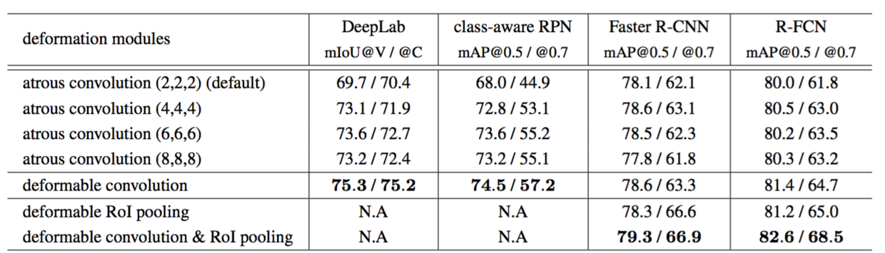
Table 3: Evaluation of our deformable modules and atrous convolution, using ResNet-101.
可变形卷积是空洞卷积的推广,如图1(c)所示。表3给出了大量的与空洞卷积的比较。
表3:我们的可变形模块与空洞卷积的评估,使用ResNet-101。
Deformable Part Models (DPM) [11] Deformable RoI pooling is similar to DPM because both methods learn the spatial deformation of object parts to maximize the classification score. Deformable RoI pooling is simpler since no spatial relations between the parts are considered.
可变形部件模型(DPM)[11]。可变形RoI池化与DPM类似,因为两种方法都可以学习目标部件的空间变形,以最大化分类得分。由于不考虑部件之间的空间关系,所以可变形RoI池化更简单。
DPM is a shallow model and has limited capability of modeling deformation. While its inference algorithm can be converted to CNNs [17] by treating the distance transform as a special pooling operation, its training is not end-to-end and involves heuristic choices such as selection of components and part sizes. In contrast, deformable ConvNets are deep and perform end-to-end training. When multiple deformable modules are stacked, the capability of modeling deformation becomes stronger.
DPM是一个浅层模型,其建模变形能力有限。虽然其推理算法可以通过将距离变换视为一个特殊的池化操作转换为CNN[17],但是它的训练不是端到端的,而是涉及启发式选择,例如选择组件和部件尺寸。相比之下,可变形ConvNets是深层的并进行端到端的训练。当多个可变形模块堆叠时,建模变形的能力变得更强。
DeepID-Net [44] It introduces a deformation constrained pooling layer which also considers part deformation for object detection. It therefore shares a similar spirit with deformable RoI pooling, but is much more complex. This work is highly engineered and based on RCNN [16]. It is unclear how to adapt it to the recent state-of-the-art object detection methods [47, 7] in an end-to-end manner.
DeepID-Net[44]。它引入了一个变形约束池化层,它也考虑了目标检测的部分变形。因此,它与可变形RoI池化共享类似的精神,但是要复杂得多。这项工作是高度工程化并基于RCNN的[16]。目前尚不清楚如何以端对端的方式将其应用于最近的最先进目标检测方法[47,7]。
Spatial manipulation in RoI pooling Spatial pyramid pooling [34] uses hand crafted pooling regions over scales. It is the predominant approach in computer vision and also used in deep learning based object detection [21, 15].
RoI池化中的空间操作。空间金字塔池化[34]在尺度上使用手工设计的池化区域。它是计算机视觉中的主要方法,也用于基于深度学习的目标检测[21,15]。
Learning the spatial layout of pooling regions has received little study. The work in [28] learns a sparse subset of pooling regions from a large over-complete set. The large set is hand engineered and the learning is not end-to-end.
很少有学习池化区域空间布局的研究。[28]中的工作从一个大型的超完备集合中学习了池化区域一个稀疏子集。大数据集是手工设计的并且学习不是端到端的。
Deformable RoI pooling is the first to learn pooling regions end-to-end in CNNs. While the regions are of the same size currently, extension to multiple sizes as in spatial pyramid pooling [34] is straightforward.
可变形RoI池化第一个在CNN中端到端地学习池化区域。虽然目前这些区域的规模相同,但像空间金字塔池化[34]那样扩展到多种尺度很简单。
Transformation invariant features and their learning There have been tremendous efforts on designing transformation invariant features. Notable examples include scale invariant feature transform (SIFT) [42] and ORB [49] (O for orientation). There is a large body of such works in the context of CNNs. The invariance and equivalence of CNN representations to image transformations are studied in [36]. Some works learn invariant CNN representations with respect to different types of transformations such as [50], scattering networks [3], convolutional jungles [32], and TI-pooling [33]. Some works are devoted for specific transformations such as symmetry [13, 9], scale [29], and rotation [53].
变换不变特征及其学习。在设计变换不变特征方面已经进行了巨大的努力。值得注意的例子包括尺度不变特征变换(SIFT)[42]和ORB[49](O为方向)。在CNN的背景下有大量这样的工作。CNN表示对图像变换的不变性和等价性在[36]中被研究。一些工作学习关于不同类型的变换(如[50],散射网络[3],卷积森林[32]和TI池化[33])的不变CNN表示。有些工作专门用于对称性[13,9],尺度[29]和旋转[53]等特定转换。
As analyzed in Section 1, in these works the transformations are known a priori. The knowledge (such as parameterization) is used to hand craft the structure of feature extraction algorithm, either fixed in such as SIFT, or with learnable parameters such as those based on CNNs. They cannot handle unknown transformations in the new tasks.
如第一部分分析的那样,在这些工作中,转换是先验的。使用知识(比如参数化)来手工设计特征提取算法的结构,或者是像SIFT那样固定的,或者用学习的参数,如基于CNN的那些。它们无法处理新任务中的未知变换。
In contrast, our deformable modules generalize various transformations (see Figure 1). The transformation invariance is learned from the target task.
相反,我们的可变形模块概括了各种转换(见图1)。从目标任务中学习变换的不变性。
Dynamic Filter [2] Similar to deformable convolution, the dynamic filters are also conditioned on the input features and change over samples. Differently, only the filter weights are learned, not the sampling locations like ours. This work is applied for video and stereo prediction.
动态滤波器[2]。与可变形卷积类似,动态滤波器也是依据输入特征并在采样上变化。不同的是,只学习滤波器权重,而不是像我们这样采样位置。这项工作适用于视频和立体声预测。
Combination of low level filters Gaussian filters and its smooth derivatives [30] are widely used to extract low level image structures such as corners, edges, T-junctions, etc. Under certain conditions, such filters form a set of basis and their linear combination forms new filters within the same group of geometric transformations, such as multiple orientations in Steerable Filters [12] and multiple scales in [45]. We note that although the term deformable kernels is used in [45], its meaning is different from ours in this work.
低级滤波器的组合。高斯滤波器及其平滑导数[30]被广泛用于提取低级图像结构,如角点,边缘,T形接点等。在某些条件下,这些滤波器形成一组基,并且它们的线性组合在同一组几何变换中形成新的滤波器,例如Steerable Filters[12]中的多个方向和[45]中多尺度。我们注意到尽管[45]中使用了可变形内核这个术语,但它的含义与我们在本文中的含义不同。
Most CNNs learn all their convolution filters from scratch. The recent work [25] shows that it could be unnecessary. It replaces the free form filters by weighted combination of low level filters (Gaussian derivatives up to 4-th order) and learns the weight coefficients. The regularization over the filter function space is shown to improve the generalization ability when training data are small.
大多数CNN从零开始学习所有的卷积滤波器。最近的工作[25]表明,这可能是没必要的。它通过低阶滤波器(高斯导数达4阶)的加权组合来代替自由形式的滤波器,并学习权重系数。通过对滤波函数空间的正则化,可以提高训练小数据量时的泛化能力。
Above works are related to ours in that, when multiple filters, especially with different scales, are combined, the resulting filter could have complex weights and resemble our deformable convolution filter. However, deformable convolution learns sampling locations instead of filter weights.
上面的工作与我们有关,当多个滤波器,尤其是不同尺度的滤波器组合时,所得到的滤波器可能具有复杂的权重,并且与我们的可变形卷积滤波器相似。但是,可变形卷积学习采样位置而不是滤波器权重。
4. Experiments
4.1. Experiment Setup and Implementation
Semantic Segmentation We use PASCAL VOC [10] and CityScapes [6]. For PASCAL VOC, there are 20 semantic categories. Following the protocols in [19, 41, 4], we use VOC 2012 dataset and the additional mask annotations in [18]. The training set includes 10, 582 images. Evaluation is performed on 1, 449 images in the validation set. For CityScapes, following the protocols in [5], training and evaluation are performed on 2, 975 images in the train set and 500 images in the validation set, respectively. There are 19 semantic categories plus a background category.
4. 实验
4.1. 实验设置和实现
语义分割。我们使用PASCAL VOC[10]和CityScapes[6]。对于PASCAL VOC,有20个语义类别。遵循[19,41,4]中的协议,我们使用VOC 2012数据集和[18]中的附加掩模注释。训练集包含10,582张图像。评估在验证集中的1,449张图像上进行。对于CityScapes,按照[5]中的协议,对训练数据集中的2,975张图像和验证集中的500张图像分别进行训练和评估。有19个语义类别加上一个背景类别。
For evaluation, we use the mean intersection-over-union (mIoU) metric defined over image pixels, following the standard protocols [10, 6]. We use mIoU@V and mIoU@C for PASCAl VOC and Cityscapes, respectively.
为了评估,我们使用在图像像素上定义的平均交集(mIoU)度量,遵循标准协议[10,6]。我们在PASCAl VOC和Cityscapes上分别使用mIoU@V和mIoU@C。
In training and inference, the images are resized to have a shorter side of $360$ pixels for PASCAL VOC and $1,024$ pixels for Cityscapes. In SGD training, one image is randomly sampled in each mini-batch. A total of 30k and 45k iterations are performed for PASCAL VOC and Cityscapes, respectively, with 8 GPUs and one mini-batch on each. The learning rates are $10^{-3}$ and $10^{-4}$ in the first $\frac{2}{3}$ and the last $\frac{1}{3}$ iterations, respectively.
在训练和推断中,PASCAL VOC中图像的大小调整为较短边有$360$个像素,Cityscapes较短边有$1,024$个像素。在SGD训练中,每个小批次数据中随机抽取一张图像。分别对PASCAL VOC和Cityscapes进行30k和45k迭代,有8个GPU每个GPU上处理一个小批次数据。前$\frac {2} {3}$次迭代和后$\frac{1}{3}$次迭代的学习率分别设为$10^{-3}$,$10^{-4}$。
Object Detection We use PASCAL VOC and COCO [39] datasets. For PASCAL VOC, following the protocol in [15], training is performed on the union of VOC 2007 trainval and VOC 2012 trainval. Evaluation is on VOC 2007 test. For COCO, following the standard protocol [39], training and evaluation are performed on the 120k images in the trainval and the 20k images in the test-dev, respectively.
目标检测。我们使用PASCAL VOC和COCO[39]数据集。对于PASCAL VOC,按照[15]中的协议,对VOC 2007 trainval和VOC 2012 trainval的并集进行培训。评估是在VOC 2007测试集上。对于COCO,遵循标准协议[39],分别对trainval中的120k张图像和test-dev中的20k张图像进行训练和评估。
For evaluation, we use the standard mean average precision (mAP) scores [10, 39]. For PASCAL VOC, we report mAP scores using IoU thresholds at 0.5 and 0.7. For COCO, we use the standard COCO metric of mAP@[0.5:0.95], as well as mAP@0.5.
为了评估,我们使用标准的平均精度均值(MAP)得分[10,39]。对于PASCAL VOC,我们使用0.5和0.7的IoU阈值报告mAP分数。对于COCO,我们使用mAP@[0.5:0.95]的标准COCO度量,以及mAP@0.5。
In training and inference, the images are resized to have a shorter side of 600 pixels. In SGD training, one image is randomly sampled in each mini-batch. For class-aware RPN, 256 RoIs are sampled from the image. For Faster R-CNN and R-FCN, 256 and 128 RoIs are sampled for the region proposal and the object detection networks, respectively. $7\times 7$ bins are adopted in RoI pooling. To facilitate the ablation experiments on VOC, we follow [38] and utilize pre-trained and fixed RPN proposals for the training of Faster R-CNN and R-FCN, without feature sharing between the region proposal and the object detection networks. The RPN network is trained separately as in the first stage of the procedure in [47]. For COCO, joint training as in [48] is performed and feature sharing is enabled for training. A total of 30k and 240k iterations are performed for PASCAL VOC and COCO, respectively, on 8 GPUs. The learning rates are set as $10^{-3}$ and $10^{-4}$ in the first $\frac{2}{3}$ and the last $\frac{1}{3}$ iterations, respectively.
在训练和推断中,图像被调整为较短边具有600像素。在SGD训练中,每个小批次中随机抽取一张图片。对于class-aware RPN,从图像中采样256个RoI。对于Faster R-CNN和R-FCN,对区域提出和目标检测网络分别采样256个和128个RoI。在ROI池化中采用$7\times 7$的组块。为了促进VOC的消融实验,我们遵循[38],并且利用预训练的和固定的RPN提出来训练Faster R-CNN和R-FCN,而区域提出和目标检测网络之间没有特征共享。RPN网络是在[47]中过程的第一阶段单独训练的。对于COCO,执行[48]中的联合训练,并且训练可以进行特征共享。在8个GPU上分别对PASCAL VOC和COCO执行30k次和240k次迭代。前$\frac {2} {3}$次迭代和后$\frac{1}{3}$次迭代的学习率分别设为$10^{-3}$,$10^{-4}$。
4.2. Ablation Study
Extensive ablation studies are performed to validate the efficacy and efficiency of our approach.
4.2. 消融研究
我们进行了广泛的消融研究来验证我们方法的功效性和有效性。
Deformable Convolution Table 1 evaluates the effect of deformable convolution using ResNet-101 feature extraction network. Accuracy steadily improves when more deformable convolution layers are used, especially for DeepLab and class-aware RPN. The improvement saturates when using 3 deformable layers for DeepLab, and 6 for others. In the remaining experiments, we use 3 in the feature extraction networks.
可变形卷积。表1使用ResNet-101特征提取网络评估可变形卷积的影响。当使用更多可变形卷积层时,精度稳步提高,特别是DeepLab和class-aware RPN。当DeepLab使用3个可变形层时,改进饱和,其它的使用6个。在其余的实验中,我们在特征提取网络中使用3个。
We empirically observed that the learned offsets in the deformable convolution layers are highly adaptive to the image content, as illustrated in Figure 5 and Figure 6. To better understand the mechanism of deformable convolution, we define a metric called effective dilation for a deformable convolution filter. It is the mean of the distances between all adjacent pairs of sampling locations in the filter. It is a rough measure of the receptive field size of the filter.
我们经验地观察到,可变形卷积层中学习到的偏移量对图像内容具有高度的自适应性,如图5和图6所示。为了更好地理解可变形卷积的机制,我们为可变形卷积滤波器定义了一个称为有效扩张的度量标准。它是滤波器中所有采样位置的相邻对之间距离的平均值。这是对滤波器的感受野大小的粗略测量。
We apply the R-FCN network with 3 deformable layers (as in Table 1) on VOC 2007 test images. We categorize the deformable convolution filters into four classes: small, medium, large, and background, according to the ground truth bounding box annotation and where the filter center is. Table 2 reports the statistics (mean and std) of the effective dilation values. It clearly shows that: 1) the receptive field sizes of deformable filters are correlated with object sizes, indicating that the deformation is effectively learned from image content; 2) the filter sizes on the background region are between those on medium and large objects, indicating that a relatively large receptive field is necessary for recognizing the background regions. These observations are consistent in different layers.
我们在VOC 2007测试图像上应用R-FCN网络,具有3个可变形层(如表1所示)。根据真实边界框标注和滤波器中心的位置,我们将可变形卷积滤波器分为四类:小,中,大和背景。表2报告了有效扩张值的统计(平均值和标准差)。它清楚地表明:1)可变形滤波器的感受野大小与目标大小相关,表明变形是从图像内容中有效学习到的; 2)背景区域上的滤波器大小介于中,大目标的滤波器之间,表明一个相对较大的感受野是识别背景区域所必需的。这些观察结果在不同层上是一致的。
The default ResNet-101 model uses atrous convolution with dilation 2 for the last three 3 × 3 convolutional layers (see Section 2.3). We further tried dilation values 4, 6, and 8 and reported the results in Table 3. It shows that: 1) accuracy increases for all tasks when using larger dilation values, indicating that the default networks have too small receptive fields; 2) the optimal dilation values vary for different tasks, e.g., 6 for DeepLab but 4 for Faster R-CNN; 3) deformable convolution has the best accuracy. These observations verify that adaptive learning of filter deformation is effective and necessary.
默认的ResNet-101模型在最后的3个3×3卷积层使用扩张为的2空洞卷积(见2.3节)。我们进一步尝试了扩张值4,6和8,并在表3中报告了结果。它表明:1)当使用较大的扩张值时,所有任务的准确度都会增加,表明默认网络的感受野太小; 2)对于不同的任务,最佳扩张值是不同的,例如,6用于DeepLab,4用于Faster R-CNN; 3)可变形卷积具有最好的精度。*这些观察结果证明了滤波器变形的自适应学习是有效和必要的。
Deformable RoI Pooling It is applicable to Faster R-CNN and R-FCN. As shown in Table 3, using it alone already produces noticeable performance gains, especially at the strict mAP@0.7 metric. When both deformable convolution and RoI Pooling are used, significant accuracy improvements are obtained.
可变形RoI池化。它适用于Faster R-CNN和R-FCN。如表3所示,单独使用它已经产生了显著的性能收益,特别是在严格的mAP@0.7度量标准下。当同时使用可变形卷积和RoI池化时,会获得显著准确性改进。
Model Complexity and Runtime Table 4 reports the model complexity and runtime of the proposed deformable ConvNets and their plain versions. Deformable ConvNets only add small overhead over model parameters and computation. This indicates that the significant performance improvement is from the capability of modeling geometric transformations, other than increasing model parameters.
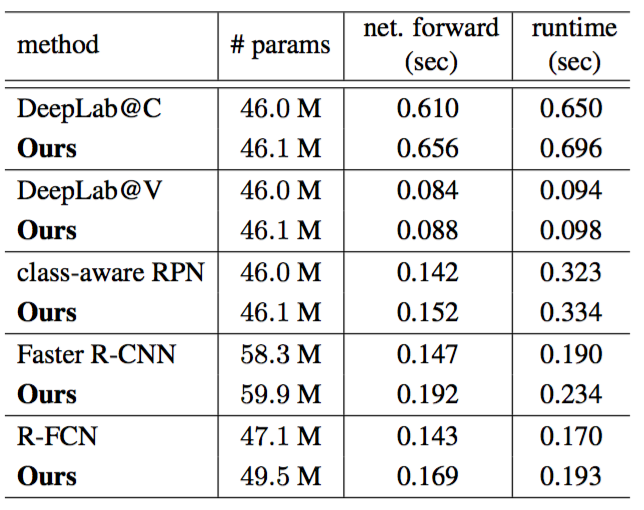
Table 4: Model complexity and runtime comparison of deformable ConvNets and the plain counterparts, using ResNet-101. The overall runtime in the last column includes image resizing, network forward, and post-processing (e.g., NMS for object detection). Runtime is counted on a workstation with Intel E5-2650 v2 CPU and Nvidia K40 GPU.
模型复杂性和运行时间。表4报告了所提出的可变形ConvNets及其普通版本的模型复杂度和运行时间。可变形ConvNets仅增加了很小的模型参数和计算量。这表明显著的性能改进来自于建模几何变换的能力,而不是增加模型参数。
表4:使用ResNet-101的可变形ConvNets和对应普通版本的模型复杂性和运行时比较。最后一列中的整体运行时间包括图像大小调整,网络前馈传播和后处理(例如,用于目标检测的NMS)。运行时间计算是在一台配备了Intel E5-2650 v2 CPU和Nvidia K40 GPU的工作站上。
4.3. Object Detection on COCO
In Table 5, we perform extensive comparison between the deformable ConvNets and the plain ConvNets for object detection on COCO test-dev set. We first experiment using ResNet-101 model. The deformable versions of class-aware RPN, Faster R-CNN and R-FCN achieve mAP@[0.5:0.95] scores of $25.8\%$, $33.1\%$, and $34.5\%$ respectively, which are $11\%$, $13\%$, and $12\%$ relatively higher than their plain-ConvNets counterparts respectively. By replacing ResNet-101 by Aligned-Inception-ResNet in Faster R-CNN and R-FCN, their plain-ConvNet baselines both improve thanks to the more powerful feature representations. And the effective performance gains brought by deformable ConvNets also hold. By further testing on multiple image scales (the image shorter side is in [480, 576, 688, 864, 1200, 1400]) and performing iterative bounding box average [14], the mAP@[0.5:0.95] scores are increased to 37.5% for the deformable version of R-FCN. Note that the performance gain of deformable ConvNets is complementary to these bells and whistles.
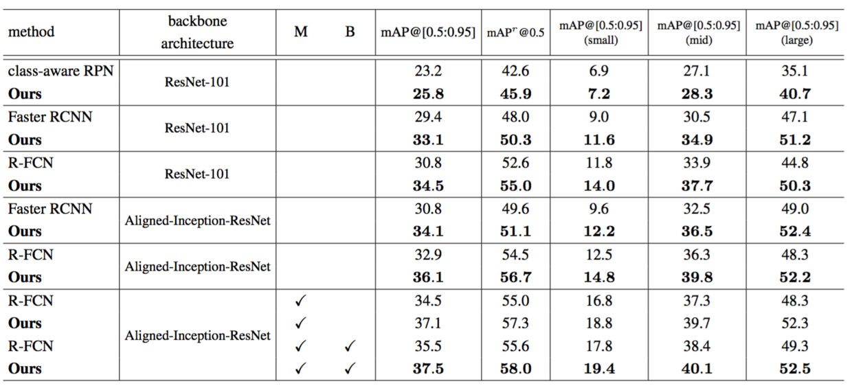
Table 5: Object detection results of deformable ConvNets v.s. plain ConvNets on COCO test-dev set. M denotes multi-scale testing, and B denotes iterative bounding box average in the table.
4.3. COCO的目标检测
在表5中,我们在COCO test-dev数据集上对用于目标检测的可变形ConvNets和普通ConvNets进行了广泛的比较。我们首先使用ResNet-101模型进行实验。class-aware RPN,Faster CNN和R-FCN的可变形版本分别获得了$25.8\%$,$33.1\%$和$34.5\%$的mAP@[0.5:0.95]分数,分别比它们对应的普通ConvNets相对高了$11\%$,$13\%$和$12\%$。通过在Faster R-CNN和R-FCN中用Aligned-Inception-ResNet取代ResNet-101,由于更强大的特征表示,它们的普通ConvNet基线都得到了提高。而可变形ConvNets带来的有效性能收益也是成立的。通过在多个图像尺度上(图像较短边在[480,576,688,864,1200,1400]内)的进一步测试,并执行迭代边界框平均[14],对于R-FCN的可变形版本,mAP@[0.5:0.95]分数增加到了37.5%。请注意,可变形ConvNets的性能增益是对这些附加功能的补充。
表5:可变形ConvNets和普通ConvNets在COCO test-dev数据集上的目标检测结果。在表中M表示多尺度测试,B表示迭代边界框平均值。
5. Conclusion
This paper presents deformable ConvNets, which is a simple, efficient, deep, and end-to-end solution to model dense spatial transformations. For the first time, we show that it is feasible and effective to learn dense spatial transformation in CNNs for sophisticated vision tasks, such as object detection and semantic segmentation.
5. 结论
本文提出了可变形ConvNets,它是一个简单,高效,深度,端到端的建模密集空间变换的解决方案。我们首次证明了在CNN中学习高级视觉任务(如目标检测和语义分割)中的密集空间变换是可行和有效的。
Acknowledgements
The Aligned-Inception-ResNet model was trained and investigated by Kaiming He, Xiangyu Zhang, Shaoqing Ren, and Jian Sun in unpublished work.
致谢
Aligned-Inception-ResNet模型由Kaiming He,Xiangyu Zhang,Shaoqing Ren和Jian Sun在未发表的工作中进行了研究和训练。
References
[1] Y.-L. Boureau, J. Ponce, and Y. LeCun. A theoretical analysis of feature pooling in visual recognition. In ICML, 2010. 1
[2] B. D. Brabandere, X. Jia, T. Tuytelaars, and L. V. Gool. Dynamic filter networks. In NIPS, 2016. 6
[3] J. Bruna and S. Mallat. Invariant scattering convolution networks. TPAMI, 2013. 6
[4] L.-C. Chen, G. Papandreou, I. Kokkinos, K. Murphy, and A. L. Yuille. Semantic image segmentation with deep convolutional nets and fully connected crfs. In ICLR, 2015. 4, 7
[5] L.-C. Chen, G. Papandreou, I. Kokkinos, K. Murphy, and A. L. Yuille. Deeplab: Semantic image segmentation with deep convolutional nets, atrous convolution, and fully connected crfs. arXiv preprint arXiv:1606.00915, 2016. 4, 6, 7
[6] M. Cordts, M. Omran, S. Ramos, T. Rehfeld, M. Enzweiler, R. Benenson, U. Franke, S. Roth, and B. Schiele. The cityscapes dataset for semantic urban scene understanding. In CVPR, 2016. 7
[7] J. Dai, Y. Li, K. He, and J. Sun. R-fcn: Object detection via region-based fully convolutional networks. In NIPS, 2016. 1, 2, 3, 4, 5, 6
[8] J. Deng, W. Dong, R. Socher, L.-J. Li, K. Li, and L. Fei-Fei. Imagenet: A large-scale hierarchical image database. In CVPR, 2009. 4, 10
[9] S. Dieleman, J. D. Fauw, and K. Kavukcuoglu. Exploiting cyclic symmetry in convolutional neural networks. arXiv preprint arXiv:1602.02660, 2016. 6
[10] M. Everingham, L. Van Gool, C. K. Williams, J. Winn, and A. Zisserman. The PASCAL Visual Object Classes (VOC) Challenge. IJCV, 2010. 7
[11] P. F. Felzenszwalb, R. B. Girshick, D. McAllester, and D. Ramanan. Object detection with discriminatively trained part-based models. TPAMI, 2010. 2, 6
[12] W. T. Freeman and E. H. Adelson. The design and use of steerable filters. TPAMI, 1991. 6
[13] R. Gens and P. M. Domingos. Deep symmetry networks. In NIPS, 2014. 6
[14] S. Gidaris and N. Komodakis. Object detection via a multiregion & semantic segmentation-aware cnn model. In ICCV, 2015. 9
[15] R. Girshick. Fast R-CNN. In ICCV, 2015. 1, 2, 3, 6, 7
[16] R. Girshick, J. Donahue, T. Darrell, and J. Malik. Rich feature hierarchies for accurate object detection and semantic segmentation. In CVPR, 2014. 1, 3, 6
[17] R. Girshick, F. Iandola, T. Darrell, and J. Malik. Deformable part models are convolutional neural networks.
[20] K. He, X. Zhang, S. Ren, and J. Sun. Aligned-inceptionresnet model, unpublished work. 4, 10
[21] K. He, X. Zhang, S. Ren, and J. Sun. Spatial pyramid pooling in deep convolutional networks for visual recognition. In ECCV, 2014. 6
[22] K. He, X. Zhang, S. Ren, and J. Sun. Deep residual learning for image recognition. In CVPR, 2016. 4, 10
[23] M. Holschneider, R. Kronland-Martinet, J. Morlet, and P. Tchamitchian. A real-time algorithm for signal analysis with the help of the wavelet transform. Wavelets: Time-Frequency Methods and Phase Space, page 289297, 1989. 6
[24] J. Huang, V. Rathod, C. Sun, M. Zhu, A. Korattikara, A. Fathi, I. Fischer, Z. Wojna, Y. Song, S. Guadarrama, and K. Murphy. Speed/accuracy trade-offs for modern convolutional object detectors. arXiv preprint arXiv:1611.10012, 2016. 4
[25] J.-H. Jacobsen, J. van Gemert, Z. Lou, and A. W.M.Smeulders. Structured receptive fields in cnns. In CVPR, 2016. 6
[26] M. Jaderberg, K. Simonyan, A. Zisserman, and K. Kavukcuoglu. Spatial transformer networks. In NIPS, 2015. 2, 5
[27] Y. Jeon and J. Kim. Active convolution: Learning the shape of convolution for image classification. In CVPR, 2017. 5
[28] Y. Jia, C. Huang, and T. Darrell. Beyond spatial pyramids: Receptive field learning for pooled image features. In CVPR, 2012. 6
[29] A. Kanazawa, A. Sharma, and D. Jacobs. Locally scale-invariant convolutional neural networks. In NIPS, 2014. 6
[30] J. J. Koenderink and A. J. van Doom. Representation of local geometry in the visual system. Biological Cybernetics, 55(6):367–375, Mar. 1987. 6
[31] A. Krizhevsky, I. Sutskever, and G. E. Hinton. Imagenet classification with deep convolutional neural networks. In NIPS, 2012. 1
[32] D. Laptev and J. M. Buhmann. Transformation-invariantcon-volutional jungles. In CVPR, 2015. 6
[33] D. Laptev, N. Savinov, J. M. Buhmann, and M. Pollefeys. Ti-pooling: transformation-invariant pooling for feature learning in convolutional neural networks. arXiv preprint arXiv:1604.06318, 2016. 6
[34] S. Lazebnik, C. Schmid, and J. Ponce. Beyond bags of features: Spatial pyramid matching for recognizing natural scene categories. In CVPR, 2006. 6
[35] Y. LeCun and Y. Bengio. Convolutional networks for images, speech, and time series. The handbook of brain theory and neural networks, 1995. 1
[36] K. Lenc and A. Vedaldi. Understanding image representations by measuring their equivariance and equivalence. In CVPR, 2015. 6
[37] C.-H. Lin and S. Lucey. Inverse compositional spatial transformer networks. arXiv preprint arXiv:1612.03897, 2016. arXiv preprint arXiv:1409.5403, 2014. 6
[18] B. Hariharan, P. Arbeláez, L. Bourdev, S. Maji, and J. Malik. 5 Semantic contours from inverse detectors. In ICCV, 2011. 7 [19] B. Hariharan, P. Arbeláez, R. Girshick, and J. Malik. Simultaneous detection and segmentation. In ECCV. 2014. 7
[38] T.-Y. Lin, P. Dollár, R. Girshick, K. He, B. Hariharan, and S. Belongie. Feature pyramid networks for object detection. In CVPR, 2017. 4, 7
[39] T.-Y. Lin, M. Maire, S. Belongie, J. Hays, P. Perona, D. Ramanan, P. Dollár, and C. L. Zitnick. Microsoft COCO: Common objects in context. In ECCV. 2014. 7
[40] W. Liu, D. Anguelov, D. Erhan, C. Szegedy, and S. Reed. Ssd: Single shot multibox detector. In ECCV, 2016. 1, 4
[41] J. Long, E. Shelhamer, and T. Darrell. Fully convolutional networks for semantic segmentation. In CVPR, 2015. 1, 6, 7
[42] D. G. Lowe. Object recognition from local scale-invariant features. In ICCV, 1999. 1, 6
[43] W. Luo, Y. Li, R. Urtasun, and R. Zemel. Understanding the effective receptive field in deep convolutional neural networks. arXiv preprint arXiv:1701.04128, 2017. 6
[44] W. Ouyang, X. Wang, X. Zeng, S. Qiu, P. Luo, Y. Tian, H. Li, S. Yang, Z. Wang, C.-C. Loy, and X. Tang. Deepid-net: Deformable deep convolutional neural networks for object detection. In CVPR, 2015. 6
[45] P. Perona. Deformable kernels for early vision. TPAMI, 1995. 6
[46] J. Redmon, S. Divvala, R. Girshick, and A. Farhadi. You only look once: Unified, real-time object detection. In CVPR, 2016. 1
[47] S. Ren, K. He, R. Girshick, and J. Sun. Faster R-CNN: Towards real-time object detection with region proposal networks. In NIPS, 2015. 1, 3, 4, 6, 7
[48] S. Ren, K. He, R. Girshick, and J. Sun. Faster R-CNN: Towards real-time object detection with region proposal networks. TPAMI, 2016. 7
[49] E. Rublee, V. Rabaud, K. Konolige, and G. Bradski. Orb: an efficient alternative to sift or surf. In ICCV, 2011. 6
[50] K. Sohn and H. Lee. Learning invariant representations with local transformations. In ICML, 2012. 6
[51] C. Szegedy, S. Ioffe, V. Vanhoucke, and A. Alemi. Inception-v4, inception-resnet and the impact of residual connections on learning. arXiv preprint arXiv:1602.07261, 2016. 4, 10
[52] C. Szegedy, S. Reed, D. Erhan, and D. Anguelov. Scalable, high-quality object detection. arXiv:1412.1441v2, 2014. 1
[53] D. E. Worrall, S. J. Garbin, D. Turmukhambetov, and G. J. Brostow. Harmonic networks: Deep translation and rotation equivariance. arXiv preprint arXiv:1612.04642, 2016. 6
[54] F. Yu and V. Koltun. Multi-scale context aggregation by dilated convolutions. In ICLR, 2016. 6
[55] F. Yu, V. Koltun, and T. Funkhouser. Dilated residual networks. In CVPR, 2017. 6

