Faster R-CNN论文翻译——中英文对照

文章作者：Tyan
博客：noahsnail.com  |  CSDN  |  简书

声明：作者翻译论文仅为学习，如有侵权请联系作者删除博文，谢谢！

翻译论文汇总：https://github.com/SnailTyan/deep-learning-papers-translation

Faster R-CNN: Towards Real-Time Object Detection with Region Proposal Networks

Abstract

State-of-the-art object detection networks depend on region proposal algorithms to hypothesize object locations. Advances like SPPnet [1] and Fast R-CNN [2] have reduced the running time of these detection networks, exposing region proposal computation as a bottleneck. In this work, we introduce a Region Proposal Network (RPN) that shares full-image convolutional features with the detection network, thus enabling nearly cost-free region proposals. An RPN is a fully convolutional network that simultaneously predicts object bounds and objectness scores at each position. The RPN is trained end-to-end to generate high-quality region proposals, which are used by Fast R-CNN for detection. We further merge RPN and Fast R-CNN into a single network by sharing their convolutional features——using the recently popular terminology of neural networks with “attention” mechanisms, the RPN component tells the unified network where to look. For the very deep VGG-16 model [3], our detection system has a frame rate of 5fps (including all steps) on a GPU, while achieving state-of-the-art object detection accuracy on PASCAL VOC 2007, 2012, and MS COCO datasets with only 300 proposals per image. In ILSVRC and COCO 2015 competitions, Faster R-CNN and RPN are the foundations of the 1st-place winning entries in several tracks. Code has been made publicly available.

摘要

最先进的目标检测网络依靠区域提出算法来假设目标的位置。SPPnet[1]和Fast R-CNN[2]等研究已经减少了这些检测网络的运行时间，使得区域提出计算成为一个瓶颈。在这项工作中，我们引入了一个区域提出网络（RPN），该网络与检测网络共享全图像的卷积特征，从而使近乎零成本的区域提出成为可能。RPN是一个全卷积网络，可以同时在每个位置预测目标边界和目标分数。RPN经过端到端的训练，可以生成高质量的区域提出，由Fast R-CNN用于检测。我们将RPN和Fast R-CNN通过共享卷积特征进一步合并为一个单一的网络——使用最近流行的具有“注意力”机制的神经网络术语，RPN组件告诉统一网络在哪里寻找。对于非常深的VGG-16模型[3]，我们的检测系统在GPU上的帧率为5fps（包括所有步骤），同时在PASCAL VOC 2007，2012和MS COCO数据集上实现了最新的目标检测精度，每个图像只有300个提出。在ILSVRC和COCO 2015竞赛中，Faster R-CNN和RPN是多个比赛中获得第一名输入的基础。代码可公开获得。

1. Introduction

Recent advances in object detection are driven by the success of region proposal methods (e.g., [4]) and region-based convolutional neural networks (R-CNNs) [5]. Although region-based CNNs were computationally expensive as originally developed in [5], their cost has been drastically reduced thanks to sharing convolutions across proposals [1], [2]. The latest incarnation, Fast R-CNN [2], achieves near real-time rates using very deep networks [3], when ignoring the time spent on region proposals. Now, proposals are the test-time computational bottleneck in state-of-the-art detection systems.

1. 引言

目标检测的最新进展是由区域提出方法（例如[4]）和基于区域的卷积神经网络（R-CNN）[5]的成功驱动的。尽管在[5]中最初开发的基于区域的CNN计算成本很高，但是由于在各种提议中共享卷积，所以其成本已经大大降低了[1]，[2]。忽略花费在区域提议上的时间，最新版本Fast R-CNN[2]利用非常深的网络[3]实现了接近实时的速率。现在，提议是最新的检测系统中测试时间的计算瓶颈。

Region proposal methods typically rely on inexpensive features and economical inference schemes. Selective Search [4], one of the most popular methods, greedily merges superpixels based on engineered low-level features. Yet when compared to efficient detection networks [2], Selective Search is an order of magnitude slower, at 2 seconds per image in a CPU implementation. EdgeBoxes [6] currently provides the best tradeoff between proposal quality and speed, at 0.2 seconds per image. Nevertheless, the region proposal step still consumes as much running time as the detection network.

区域提议方法通常依赖廉价的特征和简练的推断方案。选择性搜索[4]是最流行的方法之一，它贪婪地合并基于设计的低级特征的超级像素。然而，与有效的检测网络[2]相比，选择性搜索速度慢了一个数量级，在CPU实现中每张图像的时间为2秒。EdgeBoxes[6]目前提供了在提议质量和速度之间的最佳权衡，每张图像0.2秒。尽管如此，区域提议步骤仍然像检测网络那样消耗同样多的运行时间。

One may note that fast region-based CNNs take advantage of GPUs, while the region proposal methods used in research are implemented on the CPU, making such runtime comparisons inequitable. An obvious way to accelerate proposal computation is to re-implement it for the GPU. This may be an effective engineering solution, but re-implementation ignores the down-stream detection network and therefore misses important opportunities for sharing computation.

有人可能会注意到，基于区域的快速CNN利用GPU，而在研究中使用的区域提议方法在CPU上实现，使得运行时间比较不公平。加速区域提议计算的一个显而易见的方法是将其在GPU上重新实现。这可能是一个有效的工程解决方案，但重新实现忽略了下游检测网络，因此错过了共享计算的重要机会。

In this paper, we show that an algorithmic change——computing proposals with a deep convolutional neural network——leads to an elegant and effective solution where proposal computation is nearly cost-free given the detection network’s computation. To this end, we introduce novel Region Proposal Networks (RPNs) that share convolutional layers with state-of-the-art object detection networks [1], [2]. By sharing convolutions at test-time, the marginal cost for computing proposals is small (e.g., 10ms per image).

在本文中，我们展示了算法的变化——用深度卷积神经网络计算区域提议——导致了一个优雅和有效的解决方案，其中在给定检测网络计算的情况下区域提议计算接近领成本。为此，我们引入了新的区域提议网络（RPN），它们共享最先进目标检测网络的卷积层[1]，[2]。通过在测试时共享卷积，计算区域提议的边际成本很小（例如，每张图像10ms）。

Our observation is that the convolutional feature maps used by region-based detectors, like Fast R-CNN, can also be used for generating region proposals. On top of these convolutional features, we construct an RPN by adding a few additional convolutional layers that simultaneously regress region bounds and objectness scores at each location on a regular grid. The RPN is thus a kind of fully convolutional network (FCN) [7] and can be trained end-to-end specifically for the task for generating detection proposals.

我们的观察是，基于区域的检测器所使用的卷积特征映射，如Fast R-CNN，也可以用于生成区域提议。在这些卷积特征之上，我们通过添加一些额外的卷积层来构建RPN，这些卷积层同时在规则网格上的每个位置上回归区域边界和目标分数。因此RPN是一种全卷积网络（FCN）[7]，可以针对生成检测区域建议的任务进行端到端的训练。

RPNs are designed to efficiently predict region proposals with a wide range of scales and aspect ratios. In contrast to prevalent methods [8], [9], [1], [2] that use pyramids of images (Figure 1, a) or pyramids of filters (Figure 1, b), we introduce novel “anchor” boxes that serve as references at multiple scales and aspect ratios. Our scheme can be thought of as a pyramid of regression references (Figure 1, c), which avoids enumerating images or filters of multiple scales or aspect ratios. This model performs well when trained and tested using single-scale images and thus benefits running speed.

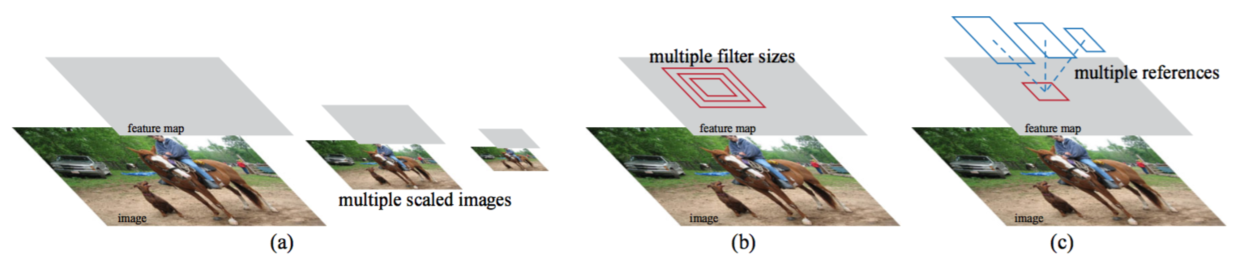
Figure 1: Different schemes for addressing multiple scales and sizes. (a) Pyramids of images and feature maps are built, and the classifier is run at all scales. (b) Pyramids of filters with multiple scales/sizes are run on the feature map. (c) We use pyramids of reference boxes in the regression functions.

RPN旨在有效预测具有广泛尺度和长宽比的区域提议。与使用图像金字塔（图1，a）或滤波器金字塔（图1，b）的流行方法[8]，[9]，[1]相比，我们引入新的“锚”盒作为多种尺度和长宽比的参考。我们的方案可以被认为是回归参考金字塔（图1，c），它避免了枚举多种比例或长宽比的图像或滤波器。这个模型在使用单尺度图像进行训练和测试时运行良好，从而有利于运行速度。

图1：解决多尺度和尺寸的不同方案。（a）构建图像和特征映射金字塔，分类器以各种尺度运行。（b）在特征映射上运行具有多个比例/大小的滤波器的金字塔。（c）我们在回归函数中使用参考边界框金字塔。

To unify RPNs with Fast R-CNN [2] object detection networks, we propose a training scheme that alternates between fine-tuning for the region proposal task and then fine-tuning for object detection, while keeping the proposals fixed. This scheme converges quickly and produces a unified network with convolutional features that are shared between both tasks.

为了将RPN与Fast R-CNN 2]目标检测网络相结合，我们提出了一种训练方案，在微调区域提议任务和微调目标检测之间进行交替，同时保持区域提议的固定。该方案快速收敛，并产生两个任务之间共享的具有卷积特征的统一网络。

We comprehensively evaluate our method on the PASCAL VOC detection benchmarks [11] where RPNs with Fast R-CNNs produce detection accuracy better than the strong baseline of Selective Search with Fast R-CNNs. Meanwhile, our method waives nearly all computational burdens of Selective Search at test-time——the effective running time for proposals is just 10 milliseconds. Using the expensive very deep models of [3], our detection method still has a frame rate of 5fps (including all steps) on a GPU, and thus is a practical object detection system in terms of both speed and accuracy. We also report results on the MS COCO dataset [12] and investigate the improvements on PASCAL VOC using the COCO data. Code has been made publicly available at https://github.com/shaoqingren/faster_rcnn (in MATLAB) and https://github.com/rbgirshick/py-faster-rcnn (in Python).

我们在PASCAL VOC检测基准数据集上[11]综合评估了我们的方法，其中具有Fast R-CNN的RPN产生的检测精度优于使用选择性搜索的Fast R-CNN的强基准。同时，我们的方法在测试时几乎免除了选择性搜索的所有计算负担——区域提议的有效运行时间仅为10毫秒。使用[3]的昂贵的非常深的模型，我们的检测方法在GPU上仍然具有5fps的帧率（包括所有步骤），因此在速度和准确性方面是实用的目标检测系统。我们还报告了在MS COCO数据集上[12]的结果，并使用COCO数据研究了在PASCAL VOC上的改进。代码可公开获得https://github.com/shaoqingren/faster_rcnn（在MATLAB中）和https://github.com/rbgirshick/py-faster-rcnn（在Python中）。

A preliminary version of this manuscript was published previously [10]. Since then, the frameworks of RPN and Faster R-CNN have been adopted and generalized to other methods, such as 3D object detection [13], part-based detection [14], instance segmentation [15], and image captioning [16]. Our fast and effective object detection system has also been built in commercial systems such as at Pinterests [17], with user engagement improvements reported.

这个手稿的初步版本是以前发表的[10]。从那时起，RPN和Faster R-CNN的框架已经被采用并推广到其他方法，如3D目标检测[13]，基于部件的检测[14]，实例分割[15]和图像标题[16]。我们快速和有效的目标检测系统也已经在Pinterest[17]的商业系统中建立了，并报告了用户参与度的提高。

In ILSVRC and COCO 2015 competitions, Faster R-CNN and RPN are the basis of several 1st-place entries [18] in the tracks of ImageNet detection, ImageNet localization, COCO detection, and COCO segmentation. RPNs completely learn to propose regions from data, and thus can easily benefit from deeper and more expressive features (such as the 101-layer residual nets adopted in [18]). Faster R-CNN and RPN are also used by several other leading entries in these competitions. These results suggest that our method is not only a cost-efficient solution for practical usage, but also an effective way of improving object detection accuracy.

在ILSVRC和COCO 2015竞赛中，Faster R-CNN和RPN是ImageNet检测，ImageNet定位，COCO检测和COCO分割中几个第一名参赛者[18]的基础。RPN完全从数据中学习提议区域，因此可以从更深入和更具表达性的特征（例如[18]中采用的101层残差网络）中轻松获益。Faster R-CNN和RPN也被这些比赛中的其他几个主要参赛者所使用。这些结果表明，我们的方法不仅是一个实用合算的解决方案，而且是一个提高目标检测精度的有效方法。

2. RELATED WORK

Object Proposals. There is a large literature on object proposal methods. Comprehensive surveys and comparisons of object proposal methods can be found in [19], [20], [21]. Widely used object proposal methods include those based on grouping super-pixels (e.g., Selective Search [4], CPMC [22], MCG [23]) and those based on sliding windows (e.g., objectness in windows [24], EdgeBoxes [6]). Object proposal methods were adopted as external modules independent of the detectors (e.g., Selective Search [4] object detectors, R-CNN [5], and Fast R-CNN [2]).

2. 相关工作

目标提议。目标提议方法方面有大量的文献。目标提议方法的综合调查和比较可以在[19]，[20]，[21]中找到。广泛使用的目标提议方法包括基于超像素分组（例如，选择性搜索[4]，CPMC[22]，MCG[23]）和那些基于滑动窗口的方法（例如窗口中的目标[24]，EdgeBoxes[6]）。目标提议方法被采用为独立于检测器（例如，选择性搜索[4]目标检测器，R-CNN[5]和Fast R-CNN[2]）的外部模块。

Deep Networks for Object Detection. The R-CNN method [5] trains CNNs end-to-end to classify the proposal regions into object categories or background. R-CNN mainly plays as a classifier, and it does not predict object bounds (except for refining by bounding box regression). Its accuracy depends on the performance of the region proposal module (see comparisons in [20]). Several papers have proposed ways of using deep networks for predicting object bounding boxes [25], [9], [26], [27]. In the OverFeat method [9], a fully-connected layer is trained to predict the box coordinates for the localization task that assumes a single object. The fully-connected layer is then turned into a convolutional layer for detecting multiple classspecific objects. The MultiBox methods [26], [27] generate region proposals from a network whose last fully-connected layer simultaneously predicts multiple class-agnostic boxes, generalizing the “single-box” fashion of OverFeat. These class-agnostic boxes are used as proposals for R-CNN [5]. The MultiBox proposal network is applied on a single image crop or multiple large image crops (e.g., 224×224), in contrast to our fully convolutional scheme. MultiBox does not share features between the proposal and detection networks. We discuss OverFeat and MultiBox in more depth later in context with our method. Concurrent with our work, the DeepMask method [28] is developed for learning segmentation proposals.

用于目标检测的深度网络。R-CNN方法[5]端到端地对CNN进行训练，将提议区域分类为目标类别或背景。R-CNN主要作为分类器，并不能预测目标边界（除了通过边界框回归进行细化）。其准确度取决于区域提议模块的性能（参见[20]中的比较）。一些论文提出了使用深度网络来预测目标边界框的方法[25]，[9]，[26]，[27]。在OverFeat方法[9]中，训练一个全连接层来预测假定单个目标定位任务的边界框坐标。然后将全连接层变成卷积层，用于检测多个类别的目标。MultiBox方法[26]，[27]从网络中生成区域提议，网络最后的全连接层同时预测多个类别不相关的边界框，并推广到OverFeat的“单边界框”方式。这些类别不可知的边界框框被用作R-CNN的提议区域[5]。与我们的全卷积方案相比，MultiBox提议网络适用于单张裁剪图像或多张大型裁剪图像（例如224×224）。MultiBox在提议区域和检测网络之间不共享特征。稍后在我们的方法上下文中会讨论OverFeat和MultiBox。与我们的工作同时进行的，DeepMask方法[28]是为学习分割提议区域而开发的。

Shared computation of convolutions [9], [1], [29], [7], [2] has been attracting increasing attention for efficient, yet accurate, visual recognition. The OverFeat paper [9] computes convolutional features from an image pyramid for classification, localization, and detection. Adaptively-sized pooling (SPP) [1] on shared convolutional feature maps is developed for efficient region-based object detection [1], [30] and semantic segmentation [29]. Fast R-CNN [2] enables end-to-end detector training on shared convolutional features and shows compelling accuracy and speed.

卷积[9]，[1]，[29]，[7]，[2]的共享计算已经越来越受到人们的关注，因为它可以有效而准确地进行视觉识别。OverFeat论文[9]计算图像金字塔的卷积特征用于分类，定位和检测。共享卷积特征映射的自适应大小池化（SPP）[1]被开发用于有效的基于区域的目标检测[1]，[30]和语义分割[29]。Fast R-CNN[2]能够对共享卷积特征进行端到端的检测器训练，并显示出令人信服的准确性和速度。

3. FASTER R-CNN

Our object detection system, called Faster R-CNN, is composed of two modules. The first module is a deep fully convolutional network that proposes regions, and the second module is the Fast R-CNN detector [2] that uses the proposed regions. The entire system is a single, unified network for object detection (Figure 2). Using the recently popular terminology of neural networks with attention [31] mechanisms, the RPN module tells the Fast R-CNN module where to look. In Section 3.1 we introduce the designs and properties of the network for region proposal. In Section 3.2 we develop algorithms for training both modules with features shared.

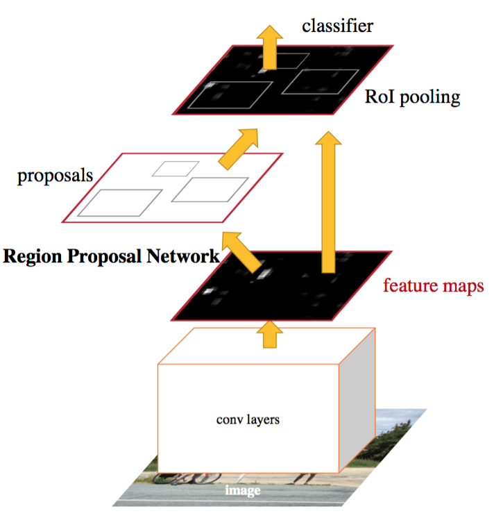
Figure 2: Faster R-CNN is a single, unified network for object detection. The RPN module serves as the ‘attention’ of this unified network.

3. FASTER R-CNN

我们的目标检测系统，称为Faster R-CNN，由两个模块组成。第一个模块是提议区域的深度全卷积网络，第二个模块是使用提议区域的Fast R-CNN检测器[2]。整个系统是一个单个的，统一的目标检测网络（图2）。使用最近流行的“注意力”[31]机制的神经网络术语，RPN模块告诉Fast R-CNN模块在哪里寻找。在第3.1节中，我们介绍了区域提议网络的设计和属性。在第3.2节中，我们开发了用于训练具有共享特征模块的算法。

图2：Faster R-CNN是一个单一，统一的目标检测网络。RPN模块作为这个统一网络的“注意力”。

3.1 Region Proposal Networks

A Region Proposal Network (RPN) takes an image (of any size) as input and outputs a set of rectangular object proposals, each with an objectness score.3 We model this process with a fully convolutional network [7], which we describe in this section. Because our ultimate goal is to share computation with a Fast R-CNN object detection network [2], we assume that both nets share a common set of convolutional layers. In our experiments, we investigate the Zeiler and Fergus model 32, which has 5 shareable convolutional layers and the Simonyan and Zisserman model 3, which has 13 shareable convolutional layers.

3.1 区域提议网络

区域提议网络（RPN）以任意大小的图像作为输入，输出一组矩形的目标提议，每个提议都有一个目标得分。我们用全卷积网络[7]对这个过程进行建模，我们将在本节进行描述。因为我们的最终目标是与Fast R-CNN目标检测网络[2]共享计算，所以我们假设两个网络共享一组共同的卷积层。在我们的实验中，我们研究了具有5个共享卷积层的Zeiler和Fergus模型[32]（ZF）和具有13个共享卷积层的Simonyan和Zisserman模型[3]（VGG-16）。

To generate region proposals, we slide a small network over the convolutional feature map output by the last shared convolutional layer. This small network takes as input an $n × n$ spatial window of the input convolutional feature map. Each sliding window is mapped to a lower-dimensional feature (256-d for ZF and 512-d for VGG, with ReLU [33] following). This feature is fed into two sibling fully-connected layers——a box-regression layer (reg) and a box-classification layer (cls). We use $n = 3$ in this paper, noting that the effective receptive field on the input image is large (171 and 228 pixels for ZF and VGG, respectively). This mini-network is illustrated at a single position in Figure 3 (left). Note that because the mini-network operates in a sliding-window fashion, the fully-connected layers are shared across all spatial locations. This architecture is naturally implemented with an n×n convolutional layer followed by two sibling 1 × 1 convolutional layers (for reg and cls, respectively).

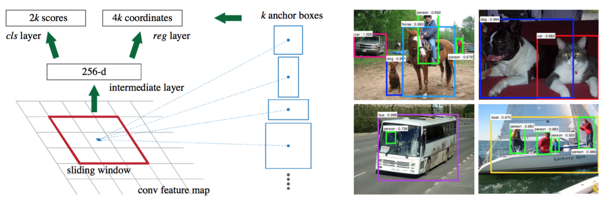
Figure 3: Left: Region Proposal Network (RPN). Right: Example detections using RPN proposals on PASCAL VOC 2007 test. Our method detects objects in a wide range of scales and aspect ratios.

为了生成区域提议，我们在最后的共享卷积层输出的卷积特征映射上滑动一个小网络。这个小网络将输入卷积特征映射的$n×n$空间窗口作为输入。每个滑动窗口映射到一个低维特征（ZF为256维，VGG为512维，后面是ReLU[33]）。这个特征被输入到两个子全连接层——一个边界框回归层（reg）和一个边界框分类层（cls）。在本文中，我们使用$n=3$，注意输入图像上的有效感受野是大的（ZF和VGG分别为171和228个像素）。图3（左）显示了这个小型网络的一个位置。请注意，因为小网络以滑动窗口方式运行，所有空间位置共享全连接层。这种架构通过一个n×n卷积层，后面是两个子1×1卷积层（分别用于reg和cls）自然地实现。

图3：左：区域提议网络（RPN）。右：在PASCAL VOC 2007测试集上使用RPN提议的示例检测。我们的方法可以检测各种尺度和长宽比的目标。

3.1.1 Anchors

At each sliding-window location, we simultaneously predict multiple region proposals, where the number of maximum possible proposals for each location is denoted as $k$. So the reg layer has $4k$ outputs encoding the coordinates of $k$ boxes, and the cls layer outputs $2k$ scores that estimate probability of object or not object for each proposal. The $k$ proposals are parameterized relative to $k$ reference boxes, which we call anchors. An anchor is centered at the sliding window in question, and is associated with a scale and aspect ratio (Figure 3, left). By default we use 3 scales and 3 aspect ratios, yielding $k=9$ anchors at each sliding position. For a convolutional feature map of a size W × H (typically ∼2,400), there are $WHk$ anchors in total.

3.1.1 锚点

在每个滑动窗口位置，我们同时预测多个区域提议，其中每个位置可能提议的最大数目表示为$k$。因此，reg层具有$4k$个输出，编码$k$个边界框的坐标，cls层输出$2k$个分数，估计每个提议是目标或不是目标的概率。相对于我们称之为锚点的$k$个参考边界框，$k$个提议是参数化的。锚点位于所讨论的滑动窗口的中心，并与一个尺度和长宽比相关（图3左）。默认情况下，我们使用3个尺度和3个长宽比，在每个滑动位置产生$k=9$个锚点。对于大小为W×H（通常约为2400）的卷积特征映射，总共有$WHk$个锚点。

Translation-Invariant Anchors

An important property of our approach is that it is translation invariant, both in terms of the anchors and the functions that compute proposals relative to the anchors. If one translates an object in an image, the proposal should translate and the same function should be able to predict the proposal in either location. This translation-invariant property is guaranteed by our method. As a comparison, the MultiBox method [27] uses k-means to generate 800 anchors, which are not translation invariant. So MultiBox does not guarantee that the same proposal is generated if an object is translated.

平移不变的锚点

我们的方法的一个重要特性是它是平移不变的，无论是在锚点还是计算相对于锚点的区域提议的函数。如果在图像中平移目标，提议应该平移，并且同样的函数应该能够在任一位置预测提议。平移不变特性是由我们的方法保证的。作为比较，MultiBox方法[27]使用k-means生成800个锚点，这不是平移不变的。所以如果平移目标，MultiBox不保证会生成相同的提议。

The translation-invariant property also reduces the model size. MultiBox has a $(4+1)\times 800$-dimensional fully-connected output layer, whereas our method has a $(4+2)\times 9$-dimensional convolutional output layer in the case of $k=9$ anchors. As a result, our output layer has $2.8\times10^4$ parameters ($512\times(4+2)\times9$ for VGG-16), two orders of magnitude fewer than MultiBox’s output layer that has $6.1\times10^6$ parameters ($1536\times(4+1)\times800$ for GoogleNet [34] in MultiBox [27]. If considering the feature projection layers, our proposal layers still have an order of magnitude fewer parameters than MultiBox. We expect our method to have less risk of overfitting on small datasets, like PASCAL VOC.

平移不变特性也减小了模型的大小。MultiBox有$(4+1)\times 800$维的全连接输出层，而我们的方法在$k=9$个锚点的情况下有$(4+2)\times 9$维的卷积输出层。因此，对于VGG-16，我们的输出层具有$2.8\times10^4$个参数（对于VGG-16为$512\times(4+2)\times9$），比MultiBox输出层的$6.1\times10^6$个参数少了两个数量级（对于MultiBox [27]中的GoogleNet[34]为$1536\times(4+1)\times800$）。如果考虑到特征投影层，我们的提议层仍然比MultiBox少一个数量级。我们期望我们的方法在PASCAL VOC等小数据集上有更小的过拟合风险。

Multi-Scale Anchors as Regression References

Our design of anchors presents a novel scheme for addressing multiple scales (and aspect ratios). As shown in Figure 1, there have been two popular ways for multi-scale predictions. The first way is based on image/feature pyramids, e.g., in DPM [8] and CNN-based methods [9], [1], [2]. The images are resized at multiple scales, and feature maps (HOG [8] or deep convolutional features [9], [1], [2]) are computed for each scale (Figure 1(a)). This way is often useful but is time-consuming. The second way is to use sliding windows of multiple scales (and/or aspect ratios) on the feature maps. For example, in DPM [8], models of different aspect ratios are trained separately using different filter sizes (such as 5×7 and 7×5). If this way is used to address multiple scales, it can be thought of as a “pyramid of filters” (Figure 1(b)). The second way is usually adopted jointly with the first way [8].

多尺度锚点作为回归参考

我们的锚点设计提出了一个新的方案来解决多尺度（和长宽比）。如图1所示，多尺度预测有两种流行的方法。第一种方法是基于图像/特征金字塔，例如DPM[8]和基于CNN的方法[9]，[1]，[2]中。图像在多个尺度上进行缩放，并且针对每个尺度（图1（a））计算特征映射（HOG[8]或深卷积特征[9]，[1]，[2]）。这种方法通常是有用的，但是非常耗时。第二种方法是在特征映射上使用多尺度（和/或长宽比）的滑动窗口。例如，在DPM[8]中，使用不同的滤波器大小（例如5×7和7×5）分别对不同长宽比的模型进行训练。如果用这种方法来解决多尺度问题，可以把它看作是一个“滤波器金字塔”（图1（b））。第二种方法通常与第一种方法联合采用[8]。

As a comparison, our anchor-based method is built on a pyramid of anchors, which is more cost-efficient. Our method classifies and regresses bounding boxes with reference to anchor boxes of multiple scales and aspect ratios. It only relies on images and feature maps of a single scale, and uses filters (sliding windows on the feature map) of a single size. We show by experiments the effects of this scheme for addressing multiple scales and sizes (Table 8).

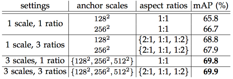
Table 8: Detection results of Faster R-CNN on PAS- CAL VOC 2007 test set using different settings of anchors. The network is VGG-16. The training data is VOC 2007 trainval. The default setting of using 3 scales and 3 aspect ratios ($69.9\%$) is the same as that in Table 3.

作为比较，我们的基于锚点方法建立在锚点金字塔上，这是更具成本效益的。我们的方法参照多尺度和长宽比的锚盒来分类和回归边界框。它只依赖单一尺度的图像和特征映射，并使用单一尺寸的滤波器（特征映射上的滑动窗口）。我们通过实验来展示这个方案解决多尺度和尺寸的效果（表8）。

表8：Faster R-CNN在PAS-CAL VOC 2007测试数据集上使用不同锚点设置的检测结果。网络是VGG-16。训练数据是VOC 2007训练集。使用3个尺度和3个长宽比（$69.9\%$）的默认设置，与表3中的相同。

Because of this multi-scale design based on anchors, we can simply use the convolutional features computed on a single-scale image, as is also done by the Fast R-CNN detector [2]. The design of multi-scale anchors is a key component for sharing features without extra cost for addressing scales.

由于这种基于锚点的多尺度设计，我们可以简单地使用在单尺度图像上计算的卷积特征，Fast R-CNN检测器也是这样做的[2]。多尺度锚点设计是共享特征的关键组件，不需要额外的成本来处理尺度。

3.1.2 Loss Function

For training RPNs, we assign a binary class label (of being an object or not) to each anchor. We assign a positive label to two kinds of anchors: (i) the anchor/anchors with the highest Intersection-over-Union (IoU) overlap with a ground-truth box, or (ii) an anchor that has an IoU overlap higher than 0.7 with any ground-truth box. Note that a single ground-truth box may assign positive labels to multiple anchors. Usually the second condition is sufficient to determine the positive samples; but we still adopt the first condition for the reason that in some rare cases the second condition may find no positive sample. We assign a negative label to a non-positive anchor if its IoU ratio is lower than 0.3 for all ground-truth boxes. Anchors that are neither positive nor negative do not contribute to the training objective.

3.1.2 损失函数

为了训练RPN，我们为每个锚点分配一个二值类别标签（是目标或不是目标）。我们给两种锚点分配一个正标签：（i）具有与实际边界框的重叠最高交并比（IoU）的锚点，或者（ii）具有与实际边界框的重叠超过0.7 IoU的锚点。注意，单个真实边界框可以为多个锚点分配正标签。通常第二个条件足以确定正样本；但我们仍然采用第一个条件，因为在一些极少数情况下，第二个条件可能找不到正样本。对于所有的真实边界框，如果一个锚点的IoU比率低于0.3，我们给非正面的锚点分配一个负标签。既不正面也不负面的锚点不会有助于训练目标函数。

With these definitions, we minimize an objective function following the multi-task loss in Fast R-CNN [2]. Our loss function for an image is defined as:$$
L(\lbrace p_i \rbrace, \lbrace t_i \rbrace) = \frac{1}{N_{cls}}\sum_i L_{cls}(p_i, p^{*}_i) \\ + \lambda\frac{1}{N_{reg}}\sum_i p^{*}_i L_{reg}(t_i, t^{*}_i).
$$Here, $i$ is the index of an anchor in a mini-batch and $p_i$ is the predicted probability of anchor $i$ being an object. The ground-truth label $p^{*}_i$ is 1 if the anchor is positive, and is 0 if the anchor is negative. $t_i$ is a vector representing the 4 parameterized coordinates of the predicted bounding box, and $t^{*}_i$ is that of the ground-truth box associated with a positive anchor. The classification loss $L_{cls}$ is log loss over two classes (object vs not object). For the regression loss, we use $L_{reg}(t_i, t^{*}_i)=R(t_i - t^{*}_i)$ where $R$ is the robust loss function (smooth $L_1$) defined in [2]. The term $p^{*}_i L_{reg}$ means the regression loss is activated only for positive anchors ($p^{*}_i=1$) and is disabled otherwise ($p^{*}_i=0$). The outputs of the cls and reg layers consist of ${p_i}$ and ${t_i}$ respectively.

根据这些定义，我们对目标函数Fast R-CNN[2]中的多任务损失进行最小化。我们对图像的损失函数定义为：$$
L(\lbrace p_i \rbrace, \lbrace t_i \rbrace) = \frac{1}{N_{cls}}\sum_i L_{cls}(p_i, p^{*}_i) \\ + \lambda\frac{1}{N_{reg}}\sum_i p^{*}_i L_{reg}(t_i, t^{*}_i).
$$其中，$i$是一个小批量数据中锚点的索引，$p_i$是锚点$i$作为目标的预测概率。如果锚点为正，真实标签$p^{*}_i$为1，如果锚点为负，则为0。$t_i$是表示预测边界框4个参数化坐标的向量，而$t^{*}_i$是与正锚点相关的真实边界框的向量。分类损失$L_{cls}$是两个类别上（目标或不是目标）的对数损失。对于回归损失，我们使用$L_{reg}(t_i, t^{*}_i)=R(t_i - t^{*}_i)$，其中$R$是在[2]中定义的鲁棒损失函数（平滑$L_1$）。项$p^{*}_i L_{reg}$表示回归损失仅对于正锚点激活，否则被禁用（$p^{*}_i=0$）。cls和reg层的输出分别由${p_i}$和${t_i}$组成。

The two terms are normalized by $N_{cls}$ and $N_{reg}$ and weighted by a balancing parameter $\lambda$. In our current implementation (as in the released code), the $cls$ term in Eqn.(1) is normalized by the mini-batch size (ie, $N_{cls}=256$) and the $reg$ term is normalized by the number of anchor locations (ie, $N_{reg} \sim 2,400$). By default we set $\lambda=10$, and thus both cls and reg terms are roughly equally weighted. We show by experiments that the results are insensitive to the values of $\lambda$ in a wide range(Table 9). We also note that the normalization as above is not required and could be simplified.

Table 9: Detection results of Faster R-CNN on PASCAL VOC 2007 test set using different values of $\lambda$ in Equation (1). The network is VGG-16. The training data is VOC 2007 trainval. The default setting of using $\lambda = 10$ ($69.9\%$) is the same as that in Table 3.

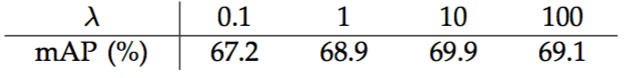
这两个项用$N_{cls}$和$N_{reg}$进行标准化，并由一个平衡参数$\lambda$加权。在我们目前的实现中（如在发布的代码中），方程（1）中的$cls$项通过小批量数据的大小（即$N_{cls}=256$）进行归一化，$reg$项根据锚点位置的数量（即，$N_{reg}\sim 24000$）进行归一化。默认情况下，我们设置$\lambda=10$，因此cls和reg项的权重大致相等。我们通过实验显示，结果对宽范围的$\lambda$值不敏感(表9)。我们还注意到，上面的归一化不是必需的，可以简化。

表9：Faster R-CNN使用方程(1)中不同的$\lambda$值在PASCAL VOC 2007测试集上的检测结果。网络是VGG-16。训练数据是VOC 2007训练集。使用$\lambda = 10$（$69.9\%$）的默认设置与表3中的相同。

For bounding box regression, we adopt the parameterizations of the 4 coordinates following [5]:
$$
t_{\textrm{x}} = (x - x_{\textrm{a}})/w_{\textrm{a}},\quad
t_{\textrm{y}} = (y - y_{\textrm{a}})/h_{\textrm{a}},\\
t_{\textrm{w}} = \log(w / w_{\textrm{a}}), \quad
t_{\textrm{h}} = \log(h / h_{\textrm{a}}),\\
t^{*}_{\textrm{x}} = (x^{*} - x_{\textrm{a}})/w_{\textrm{a}},\quad
t^{*}_{\textrm{y}} = (y^{*} - y_{\textrm{a}})/h_{\textrm{a}},\\
t^{*}_{\textrm{w}} = \log(w^{*} / w_{\textrm{a}}),\quad
t^{*}_{\textrm{h}} = \log(h^{*} / h_{\textrm{a}}),
$$ where $x$, $y$, $w$, and $h$ denote the box’s center coordinates and its width and height. Variables $x$, $x_{\textrm{a}}$, and $x^{*}$ are for the predicted box, anchor box, and ground-truth box respectively (likewise for $y, w, h$). This can be thought of as bounding-box regression from an anchor box to a nearby ground-truth box.

对于边界框回归，我们采用[5]中的4个坐标参数化：$$
t_{\textrm{x}} = (x - x_{\textrm{a}})/w_{\textrm{a}},\quad
t_{\textrm{y}} = (y - y_{\textrm{a}})/h_{\textrm{a}},\\
t_{\textrm{w}} = \log(w / w_{\textrm{a}}), \quad
t_{\textrm{h}} = \log(h / h_{\textrm{a}}),\\
t^{*}_{\textrm{x}} = (x^{*} - x_{\textrm{a}})/w_{\textrm{a}},\quad
t^{*}_{\textrm{y}} = (y^{*} - y_{\textrm{a}})/h_{\textrm{a}},\\
t^{*}_{\textrm{w}} = \log(w^{*} / w_{\textrm{a}}),\quad
t^{*}_{\textrm{h}} = \log(h^{*} / h_{\textrm{a}}),
$$ 其中，$x$，$y$，$w$和$h$表示边界框的中心坐标及其宽和高。变量$x$，$x_{\textrm{a}}$和$x^{*}$分别表示预测边界框，锚盒和实际边界框（类似于$y, w, h$）。这可以被认为是从锚盒到邻近的实际边界框的回归。

Nevertheless, our method achieves bounding-box regression by a different manner from previous RoI-based (Region of Interest) methods [1], [2]. In [1], [2], bounding-box regression is performed on features pooled from arbitrarily sized RoIs, and the regression weights are shared by all region sizes. In our formulation, the features used for regression are of the same spatial size (3 × 3) on the feature maps. To account for varying sizes, a set of $k$ bounding-box regressors are learned. Each regressor is responsible for one scale and one aspect ratio, and the $k$ regressors do not share weights. As such, it is still possible to predict boxes of various sizes even though the features are of a fixed size/scale, thanks to the design of anchors.

然而，我们的方法通过与之前的基于RoI（感兴趣区域）方法[1]，[2]不同的方式来实现边界框回归。在[1]，[2]中，对任意大小的RoI池化的特征执行边界框回归，并且回归权重由所有区域大小共享。在我们的公式中，用于回归的特征在特征映射上具有相同的空间大小（3×3）。为了说明不同的大小，学习一组$k$个边界框回归器。每个回归器负责一个尺度和一个长宽比，而$k$个回归器不共享权重。因此，由于锚点的设计，即使特征具有固定的尺度/比例，仍然可以预测各种尺寸的边界框。

3.1.3 Training RPNs

The RPN can be trained end-to-end by back-propagation and stochastic gradient descent (SGD) [35]. We follow the “image-centric” sampling strategy from [2] to train this network. Each mini-batch arises from a single image that contains many positive and negative example anchors. It is possible to optimize for the loss functions of all anchors, but this will bias towards negative samples as they are dominate. Instead, we randomly sample 256 anchors in an image to compute the loss function of a mini-batch, where the sampled positive and negative anchors have a ratio of up to 1:1. If there are fewer than 128 positive samples in an image, we pad the mini-batch with negative ones.

3.1.3 训练RPN

RPN可以通过反向传播和随机梯度下降（SGD）进行端对端训练[35]。我们遵循[2]的“以图像为中心”的采样策略来训练这个网络。每个小批量数据都从包含许多正面和负面示例锚点的单张图像中产生。对所有锚点的损失函数进行优化是可能的，但是这样会偏向于负样本，因为它们是占主导地位的。取而代之的是，我们在图像中随机采样256个锚点，计算一个小批量数据的损失函数，其中采样的正锚点和负锚点的比率可达1:1。如果图像中的正样本少于128个，我们使用负样本填充小批量数据。

We randomly initialize all new layers by drawing weights from a zero-mean Gaussian distribution with standard deviation 0.01. All other layers (i.e., the shared convolutional layers) are initialized by pre-training a model for ImageNet classification [36], as is standard practice [5]. We tune all layers of the ZF net, and conv3_1 and up for the VGG net to conserve memory [2]. We use a learning rate of 0.001 for 60k mini-batches, and 0.0001 for the next 20k mini-batches on the PASCAL VOC dataset. We use a momentum of 0.9 and a weight decay of 0.0005 [37]. Our implementation uses Caffe [38].

我们通过从标准方差为0.01的零均值高斯分布中提取权重来随机初始化所有新层。所有其他层（即共享卷积层）通过预训练的ImageNet分类模型[36]来初始化，如同标准实践[5]。我们调整ZF网络的所有层，以及VGG网络的conv3_1及其之上的层以节省内存[2]。对于60k的小批量数据，我们使用0.001的学习率，对于PASCAL VOC数据集中的下一个20k小批量数据，使用0.0001。我们使用0.9的动量和0.0005的重量衰减[37]。我们的实现使用Caffe[38]。

3.2 Sharing Features for RPN and Fast R-CNN

Thus far we have described how to train a network for region proposal generation, without considering the region-based object detection CNN that will utilize these proposals. For the detection network, we adopt Fast R-CNN [2]. Next we describe algorithms that learn a unified network composed of RPN and Fast R-CNN with shared convolutional layers (Figure 2).

3.2 RPN和Fast R-CNN共享特征

到目前为止，我们已经描述了如何训练用于区域提议生成的网络，没有考虑将利用这些提议的基于区域的目标检测CNN。对于检测网络，我们采用Fast R-CNN[2]。接下来我们介绍一些算法，学习由RPN和Fast R-CNN组成的具有共享卷积层的统一网络（图2）。

Both RPN and Fast R-CNN, trained independently, will modify their convolutional layers in different ways. We therefore need to develop a technique that allows for sharing convolutional layers between the two networks, rather than learning two separate networks. We discuss three ways for training networks with features shared:

独立训练的RPN和Fast R-CNN将以不同的方式修改卷积层。因此，我们需要开发一种允许在两个网络之间共享卷积层的技术，而不是学习两个独立的网络。我们讨论三个方法来训练具有共享特征的网络：

(i) Alternating training. In this solution, we first train RPN, and use the proposals to train Fast R-CNN. The network tuned by Fast R-CNN is then used to initialize RPN, and this process is iterated. This is the solution that is used in all experiments in this paper.

（一）交替训练。在这个解决方案中，我们首先训练RPN，并使用这些提议来训练Fast R-CNN。由Fast R-CNN微调的网络然后被用于初始化RPN，并且重复这个过程。这是本文所有实验中使用的解决方案。

(ii) Approximate joint training. In this solution, the RPN and Fast R-CNN networks are merged into one network during training as in Figure 2. In each SGD iteration, the forward pass generates region proposals which are treated just like fixed, pre-computed proposals when training a Fast R-CNN detector. The backward propagation takes place as usual, where for the shared layers the backward propagated signals from both the RPN loss and the Fast R-CNN loss are combined. This solution is easy to implement. But this solution ignores the derivative w.r.t. the proposal boxes’ coordinates that are also network responses, so is approximate. In our experiments, we have empirically found this solver produces close results, yet reduces the training time by about $25-50\%$ comparing with alternating training. This solver is included in our released Python code.

（二）近似联合训练。在这个解决方案中，RPN和Fast R-CNN网络在训练期间合并成一个网络，如图2所示。在每次SGD迭代中，前向传递生成区域提议，在训练Fast R-CNN检测器将这看作是固定的、预计算的提议。反向传播像往常一样进行，其中对于共享层，组合来自RPN损失和Fast R-CNN损失的反向传播信号。这个解决方案很容易实现。但是这个解决方案忽略了关于提议边界框的坐标（也是网络响应）的导数，因此是近似的。在我们的实验中，我们实验发现这个求解器产生了相当的结果，与交替训练相比，训练时间减少了大约$25-50\%$。这个求解器包含在我们发布的Python代码中。

(iii) Non-approximate joint training. As discussed above, the bounding boxes predicted by RPN are also functions of the input. The RoI pooling layer [2] in Fast R-CNN accepts the convolutional features and also the predicted bounding boxes as input, so a theoretically valid backpropagation solver should also involve gradients w.r.t. the box coordinates. These gradients are ignored in the above approximate joint training. In a non-approximate joint training solution, we need an RoI pooling layer that is differentiable w.r.t. the box coordinates. This is a nontrivial problem and a solution can be given by an “RoI warping” layer as developed in [15], which is beyond the scope of this paper.

（三）非近似的联合训练。如上所述，由RPN预测的边界框也是输入的函数。Fast R-CNN中的RoI池化层[2]接受卷积特征以及预测的边界框作为输入，所以理论上有效的反向传播求解器也应该包括关于边界框坐标的梯度。在上述近似联合训练中，这些梯度被忽略。在一个非近似的联合训练解决方案中，我们需要一个关于边界框坐标可微分的RoI池化层。这是一个重要的问题，可以通过[15]中提出的“RoI扭曲”层给出解决方案，这超出了本文的范围。

4-Step Alternating Training. In this paper, we adopt a pragmatic 4-step training algorithm to learn shared features via alternating optimization. In the first step, we train the RPN as described in Section 3.1.3. This network is initialized with an ImageNet-pre-trained model and fine-tuned end-to-end for the region proposal task. In the second step, we train a separate detection network by Fast R-CNN using the proposals generated by the step-1 RPN. This detection network is also initialized by the ImageNet-pre-trained model. At this point the two networks do not share convolutional layers. In the third step, we use the detector network to initialize RPN training, but we fix the shared convolutional layers and only fine-tune the layers unique to RPN. Now the two networks share convolutional layers. Finally, keeping the shared convolutional layers fixed, we fine-tune the unique layers of Fast R-CNN. As such, both networks share the same convolutional layers and form a unified network. A similar alternating training can be run for more iterations, but we have observed negligible improvements.

四步交替训练。在本文中，我们采用实用的四步训练算法，通过交替优化学习共享特征。在第一步中，我们按照3.1.3节的描述训练RPN。该网络使用ImageNet的预训练模型进行初始化，并针对区域提议任务进行了端到端的微调。在第二步中，我们使用由第一步RPN生成的提议，由Fast R-CNN训练单独的检测网络。该检测网络也由ImageNet的预训练模型进行初始化。此时两个网络不共享卷积层。在第三步中，我们使用检测器网络来初始化RPN训练，但是我们修正共享的卷积层，并且只对RPN特有的层进行微调。现在这两个网络共享卷积层。最后，保持共享卷积层的固定，我们对Fast R-CNN的独有层进行微调。因此，两个网络共享相同的卷积层并形成统一的网络。类似的交替训练可以运行更多的迭代，但是我们只观察到可以忽略的改进。

3.3 Implementation Details

We train and test both region proposal and object detection networks on images of a single scale [1], [2]. We re-scale the images such that their shorter side is $s = 600$ pixels [2]. Multi-scale feature extraction (using an image pyramid) may improve accuracy but does not exhibit a good speed-accuracy trade-off [2]. On the re-scaled images, the total stride for both ZF and VGG nets on the last convolutional layer is 16 pixels, and thus is ∼10 pixels on a typical PASCAL image before resizing (∼500×375). Even such a large stride provides good results, though accuracy may be further improved with a smaller stride.

3.3 实现细节

我们在单尺度图像上训练和测试区域提议和目标检测网络[1]，[2]。我们重新缩放图像，使得它们的短边是$s=600$像素[2]。多尺度特征提取（使用图像金字塔）可能会提高精度，但不会表现出速度与精度的良好折衷[2]。在重新缩放的图像上，最后卷积层上的ZF和VGG网络的总步长为16个像素，因此在调整大小（〜500×375）之前，典型的PASCAL图像上的总步长为〜10个像素。即使如此大的步长也能提供良好的效果，尽管步幅更小，精度可能会进一步提高。

For anchors, we use 3 scales with box areas of $128^2$, $256^2$, and $512^2$ pixels, and 3 aspect ratios of 1:1, 1:2, and 2:1. These hyper-parameters are not carefully chosen for a particular dataset, and we provide ablation experiments on their effects in the next section. As discussed, our solution does not need an image pyramid or filter pyramid to predict regions of multiple scales, saving considerable running time. Figure 3 (right) shows the capability of our method for a wide range of scales and aspect ratios. Table 1 shows the learned average proposal size for each anchor using the ZF net. We note that our algorithm allows predictions that are larger than the underlying receptive field. Such predictions are not impossible—one may still roughly infer the extent of an object if only the middle of the object is visible.

Table 1: the learned average proposal size for each anchor using the ZF net (numbers for $s = 600$).

对于锚点，我们使用了3个尺度，边界框面积分别为$128^2$，$256^2$和$512^2$个像素，以及1:1，1:2和2:1的长宽比。这些超参数不是针对特定数据集仔细选择的，我们将在下一节中提供有关其作用的消融实验。如上所述，我们的解决方案不需要图像金字塔或滤波器金字塔来预测多个尺度的区域，节省了大量的运行时间。图3（右）显示了我们的方法在广泛的尺度和长宽比方面的能力。表1显示了使用ZF网络的每个锚点学习到的平均提议大小。我们注意到，我们的算法允许预测比基础感受野更大。这样的预测不是不可能的——如果只有目标的中间部分是可见的，那么仍然可以粗略地推断出目标的范围。

表1：使用ZF网络的每个锚点学习到的平均提议大小（$s=600$的数字）。

The anchor boxes that cross image boundaries need to be handled with care. During training, we ignore all cross-boundary anchors so they do not contribute to the loss. For a typical $1000 \times 600$ image, there will be roughly 20000 ($\approx 60 \times 40 \times 9$) anchors in total. With the cross-boundary anchors ignored, there are about 6000 anchors per image for training. If the boundary-crossing outliers are not ignored in training, they introduce large, difficult to correct error terms in the objective, and training does not converge. During testing, however, we still apply the fully convolutional RPN to the entire image. This may generate cross-boundary proposal boxes, which we clip to the image boundary.

跨越图像边界的锚盒需要小心处理。在训练过程中，我们忽略了所有的跨界锚点，所以不会造成损失。对于一个典型的$1000 \times 600$的图片，总共将会有大约20000（$\approx 60 \times 40 \times 9$）个锚点。跨界锚点被忽略，每张图像约有6000个锚点用于训练。如果跨界异常值在训练中不被忽略，则会在目标函数中引入大的，难以纠正的误差项，且训练不会收敛。但在测试过程中，我们仍然将全卷积RPN应用于整张图像。这可能会产生跨边界的提议边界框，我们剪切到图像边界。

Some RPN proposals highly overlap with each other. To reduce redundancy, we adopt non-maximum suppression (NMS) on the proposal regions based on their cls scores. We fix the IoU threshold for NMS at 0.7, which leaves us about 2000 proposal regions per image. As we will show, NMS does not harm the ultimate detection accuracy, but substantially reduces the number of proposals. After NMS, we use the top-N ranked proposal regions for detection. In the following, we train Fast R-CNN using 2000 RPN proposals, but evaluate different numbers of proposals at test-time.

一些RPN提议互相之间高度重叠。为了减少冗余，我们在提议区域根据他们的cls分数采取非极大值抑制（NMS）。我们将NMS的IoU阈值固定为0.7，这就给每张图像留下了大约2000个提议区域。正如我们将要展示的那样，NMS不会损害最终的检测准确性，但会大大减少提议的数量。在NMS之后，我们使用前N个提议区域来进行检测。接下来，我们使用2000个RPN提议对Fast R-CNN进行训练，但在测试时评估不同数量的提议。

4. EXPERIMENTS

4.1 Experiments on PASCAL VOC

We comprehensively evaluate our method on the PASCAL VOC 2007 detection benchmark [11]. This dataset consists of about 5k trainval images and 5k test images over 20 object categories. We also provide results on the PASCAL VOC 2012 benchmark for a few models. For the ImageNet pre-trained network, we use the “fast” version of ZF net [32] that has 5 convolutional layers and 3 fully-connected layers, and the public VGG-16 model [3] that has 13 convolutional layers and 3 fully-connected layers. We primarily evaluate detection mean Average Precision (mAP), because this is the actual metric for object detection (rather than focusing on object proposal proxy metrics).

4. 实验

4.1 PASCAL VOC上的实验

我们在PASCAL VOC 2007检测基准数据集[11]上全面评估了我们的方法。这个数据集包含大约5000张训练评估图像和在20个目标类别上的5000张测试图像。我们还提供了一些模型在PASCAL VOC 2012基准数据集上的测试结果。对于ImageNet预训练网络，我们使用具有5个卷积层和3个全连接层的ZF网络[32]的“快速”版本以及具有13个卷积层和3个全连接层的公开的VGG-16模型[3]。我们主要评估检测的平均精度均值（mAP），因为这是检测目标的实际指标（而不是关注目标提议代理度量）。

Table 2 (top) shows Fast R-CNN results when trained and tested using various region proposal methods. These results use the ZF net. For Selective Search (SS) [4], we generate about 2000 proposals by the “fast” mode. For EdgeBoxes (EB) [6], we generate the proposals by the default EB setting tuned for 0.7 IoU. SS has an mAP of $58.7\%$ and EB has an mAP of $58.6\%$ under the Fast R-CNN framework. RPN with Fast R-CNN achieves competitive results, with an mAP of $59.9\%$ while using up to 300 proposals. Using RPN yields a much faster detection system than using either SS or EB because of shared convolutional computations; the fewer proposals also reduce the region-wise fully-connected layers’ cost (Table 5).

Table 2: Detection results on PASCAL VOC 2007 test set (trained on VOC 2007 trainval). The detectors are Fast R-CNN with ZF, but using various proposal methods for training and testing.

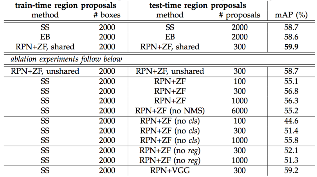
Table 5: Timing (ms) on a K40 GPU, except SS proposal is evaluated in a CPU. “Region-wise” includes NMS, pooling, fully-connected, and softmax layers. See our released code for the profiling of running time.

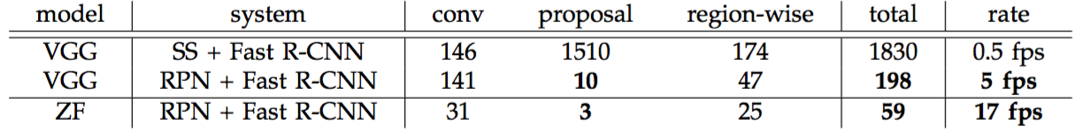
表2（顶部）显示了使用各种区域提议方法进行训练和测试的Fast R-CNN结果。这些结果使用ZF网络。对于选择性搜索（SS）[4]，我们通过“快速”模式生成约2000个提议。对于EdgeBoxes（EB）[6]，我们通过调整0.7 IoU的默认EB设置生成提议。SS在Fast R-CNN框架下的mAP为$58.7\%$，EB的mAP为$58.6\%$。RPN与Fast R-CNN取得了有竞争力的结果，使用多达300个提议，mAP为$59.9\%$。由于共享卷积计算，使用RPN比使用SS或EB产生了更快的检测系统；较少的建议也减少了区域方面的全连接层成本（表5）。

表2：PASCAL VOC 2007测试集上的检测结果（在VOC 2007训练评估集上进行了训练）。检测器是带有ZF的Fast R-CNN，但使用各种提议方法进行训练和测试。

表5：K40 GPU上的时间（ms），除了SS提议是在CPU上评估。“区域方面”包括NMS，池化，全连接和softmax层。查看我们发布的代码来分析运行时间。

Ablation Experiments on RPN. To investigate the behavior of RPNs as a proposal method, we conducted several ablation studies. First, we show the effect of sharing convolutional layers between the RPN and Fast R-CNN detection network. To do this, we stop after the second step in the 4-step training process. Using separate networks reduces the result slightly to $58.7\%$ (RPN+ZF, unshared, Table 2). We observe that this is because in the third step when the detector-tuned features are used to fine-tune the RPN, the proposal quality is improved.

RPN上的消融实验。为了研究RPN作为提议方法的性能，我们进行了几项消融研究。首先，我们显示了RPN和Fast R-CNN检测网络共享卷积层的效果。为此，我们在四步训练过程的第二步之后停止训练。使用单独的网络将结果略微减少到$58.7\%$（RPN+ZF，非共享，表2）。我们观察到，这是因为在第三步中，当使用检测器调整的特征来微调RPN时，提议质量得到了改善。

Next, we disentangle the RPN’s influence on training the Fast R-CNN detection network. For this purpose, we train a Fast R-CNN model by using the 2000 SS proposals and ZF net. We fix this detector and evaluate the detection mAP by changing the proposal regions used at test-time. In these ablation experiments, the RPN does not share features with the detector.

接下来，我们分析RPN对训练Fast R-CNN检测网络的影响。为此，我们通过使用2000个SS提议和ZF网络来训练Fast R-CNN模型。我们固定这个检测器，并通过改变测试时使用的提议区域来评估检测的mAP。在这些消融实验中，RPN不与检测器共享特征。

Replacing SS with 300 RPN proposals at test-time leads to an mAP of $56.8\%$. The loss in mAP is because of the inconsistency between the training/testing proposals. This result serves as the baseline for the following comparisons.

在测试阶段用300个RPN提议替换SS提议得到了$56.8\%$的MAP。mAP的损失是因为训练/测试提议不一致。这个结果作为以下比较的基准。

Somewhat surprisingly, the RPN still leads to a competitive result ($55.1\%$) when using the top-ranked 100 proposals at test-time, indicating that the top-ranked RPN proposals are accurate. On the other extreme, using the top-ranked 6000 RPN proposals (without NMS) has a comparable mAP ($55.2\%$), suggesting NMS does not harm the detection mAP and may reduce false alarms.

有些令人惊讶的是，RPN在测试时使用排名最高的100个提议仍然会导致有竞争力的结果（$55.1\%$），表明排名靠前的RPN提议是准确的。相反的，使用排名靠前的6000个RPN提议（无NMS）具有相当的mAP（$55.2\%$），这表明NMS不会损害检测mAP并可能减少误报。

Next, we separately investigate the roles of RPN’s cls and reg outputs by turning off either of them at test-time. When the cls layer is removed at test-time (thus no NMS/ranking is used), we randomly sample $N$ proposals from the unscored regions. The mAP is nearly unchanged with $N=1000$ ($55.8\%$), but degrades considerably to $44.6\%$ when $N=100$. This shows that the cls scores account for the accuracy of the highest ranked proposals.

接下来，我们通过在测试时分别关闭RPN的cls和reg输出来调查RPN的作用。当cls层在测试时被移除（因此不使用NMS/排名），我们从未得分的区域中随机采样$N$个提议。当$N=1000$($55.8\
%$)时，mAP几乎没有变化，但是当$N=100$时，会大大降低到$44.6\%$。这表明cls分数考虑了排名最高的提议的准确性。

On the other hand, when the reg layer is removed at test-time (so the proposals become anchor boxes), the mAP drops to $52.1\%$. This suggests that the high-quality proposals are mainly due to the regressed box bounds. The anchor boxes, though having multiple scales and aspect ratios, are not sufficient for accurate detection.

另一方面，当在测试阶段移除reg层（所以提议变成锚盒）时，mAP将下降到$52.1\%$。这表明高质量的提议主要是由于回归的边界框。锚盒虽然具有多个尺度和长宽比，但不足以进行准确的检测。

We also evaluate the effects of more powerful networks on the proposal quality of RPN alone. We use VGG-16 to train the RPN, and still use the above detector of SS+ZF. The mAP improves from $56.8\%$ (using RPN+ZF) to $59.2\%$ (using RPN+VGG). This is a promising result, because it suggests that the proposal quality of RPN+VGG is better than that of RPN+ZF. Because proposals of RPN+ZF are competitive with SS (both are $58.7\%$ when consistently used for training and testing), we may expect RPN+VGG to be better than SS. The following experiments justify this hypothesis.

我们还单独评估了更强大的网络对RPN提议质量的影响。我们使用VGG-16来训练RPN，仍然使用上述的SS+ZF检测器。mAP从$56.8\%$（使用RPN+ZF）提高到$59.2\%$（使用RPN+VGG）。这是一个很有希望的结果，因为这表明RPN+VGG的提议质量要好于RPN+ZF。由于RPN+ZF的提议与SS具有竞争性（当一致用于训练和测试时，都是$58.7\%$），所以我们可以预期RPN+VGG比SS更好。以下实验验证了这个假设。

Performance of VGG-16. Table 3 shows the results of VGG-16 for both proposal and detection. Using RPN+VGG, the result is $68.5\%$ for unshared features, slightly higher than the SS baseline. As shown above, this is because the proposals generated by RPN+VGG are more accurate than SS. Unlike SS that is pre-defined, the RPN is actively trained and benefits from better networks. For the feature-shared variant, the result is $69.9\%$——better than the strong SS baseline, yet with nearly cost-free proposals. We further train the RPN and detection network on the union set of PASCAL VOC 2007 trainval and 2012 trainval. The mAP is $73.2\%$. Figure 5 shows some results on the PASCAL VOC 2007 test set. On the PASCAL VOC 2012 test set (Table 4), our method has an mAP of $70.4\%$ trained on the union set of VOC 2007 trainval+test and VOC 2012 trainval. Table 6 and Table 7 show the detailed numbers.

Table 3: Detection results on PASCAL VOC 2007 test set. The detector is Fast R-CNN and VGG-16. Training data: “07”: VOC 2007 trainval, “07+12”: union set of VOC 2007 trainval and VOC 2012 trainval. For RPN, the train-time proposals for Fast R-CNN are 2000. †: this number was reported in [2]; using the repository provided by this paper, this result is higher (68.1).

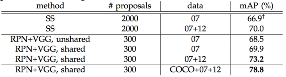
Table 4: Detection results on PASCAL VOC 2012 test set. The detector is Fast R-CNN and VGG-16. Training data: “07”: VOC 2007 trainval, “07++12”: union set of VOC 2007 trainval+test and VOC 2012 trainval. For RPN, the train-time proposals for Fast R-CNN are 2000. †: http://host.robots.ox.ac.uk:8080/anonymous/HZJTQA.html. ‡: http://host.robots.ox.ac.uk:8080/anonymous/YNPLXB.html. §: http://host.robots.ox.ac.uk:8080/anonymous/XEDH10.html.

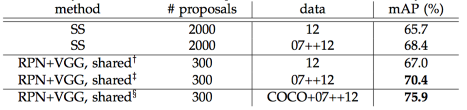
Table 6: Results on PASCAL VOC 2007 test set with Fast R-CNN detectors and VGG-16. For RPN, the train-time proposals for Fast R-CNN are 2000. ${RPN}^*$ denotes the unsharing feature version.

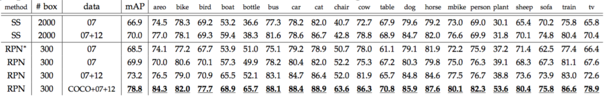
Table 7: Results on PASCAL VOC 2012 test set with Fast R-CNN detectors and VGG-16. For RPN, the train-time proposals for Fast R-CNN are 2000.

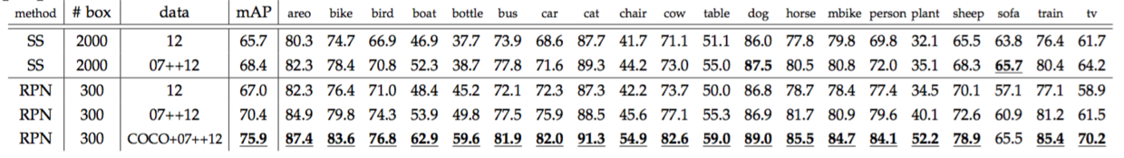
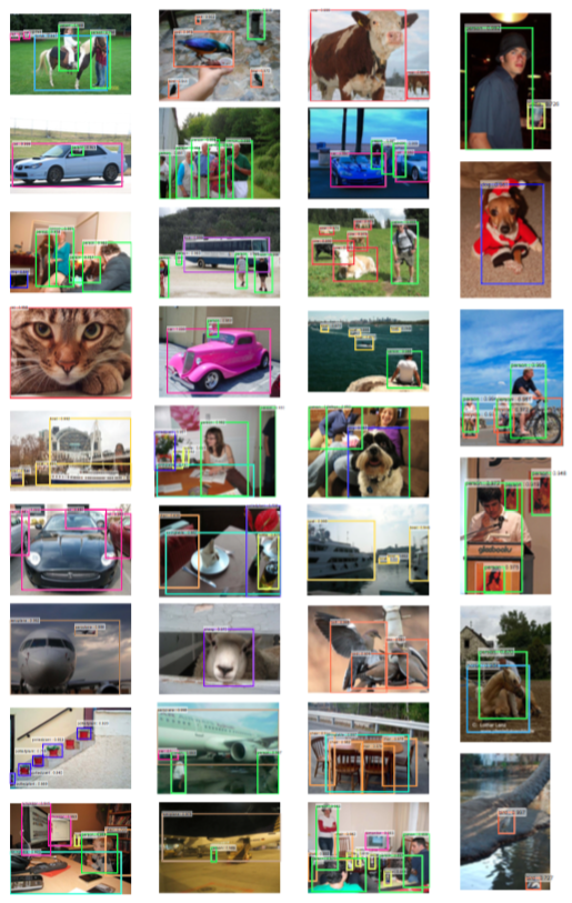
Figure 5: Selected examples of object detection results on the PASCAL VOC 2007 test set using the Faster R-CNN system. The model is VGG-16 and the training data is 07+12 trainval ($73.2\%$ mAP on the 2007 test set). Our method detects objects of a wide range of scales and aspect ratios. Each output box is associated with a category label and a softmax score in [0, 1]. A score threshold of 0.6 is used to display these images. The running time for obtaining these results is 198ms per image, including all steps.

VGG-16的性能。表3显示了VGG-16的提议和检测结果。使用RPN+VGG，非共享特征的结果是$68.5\%$，略高于SS的基准。如上所示，这是因为RPN+VGG生成的提议比SS更准确。与预先定义的SS不同，RPN是主动训练的并从更好的网络中受益。对于特性共享的变种，结果是$69.9\%$——比强壮的SS基准更好，但几乎是零成本的提议。我们在PASCAL VOC 2007和2012的训练评估数据集上进一步训练RPN和检测网络。该mAP是$73.2\%$。图5显示了PASCAL VOC 2007测试集的一些结果。在PASCAL VOC 2012测试集（表4）中，我们的方法在VOC 2007的trainval+test和VOC 2012的trainval的联合数据集上训练的模型取得了$70.4\%$的mAP。表6和表7显示了详细的数字。

表3：PASCAL VOC 2007测试集的检测结果。检测器是Fast R-CNN和VGG-16。训练数据：“07”：VOC 2007 trainval，“07 + 12”：VOC 2007 trainval和VOC 2012 trainval的联合训练集。对于RPN，训练时Fast R-CNN的提议数量为2000。†：[2]中报道的数字；使用本文提供的仓库，这个结果更高（68.1）。

表4：PASCAL VOC 2012测试集的检测结果。检测器是Fast R-CNN和VGG-16。训练数据：“07”：VOC 2007 trainval，“07 + 12”：VOC 2007 trainval和VOC 2012 trainval的联合训练集。对于RPN，训练时Fast R-CNN的提议数量为2000。†：http://host.robots.ox.ac.uk:8080/anonymous/HZJTQA.html。‡：http://host.robots.ox.ac.uk:8080/anonymous/YNPLXB.html。§：http://host.robots.ox.ac.uk:8080/anonymous/XEDH10.html。

表6：使用Fast R-CNN检测器和VGG-16在PASCAL VOC 2007测试集上的结果。对于RPN，训练时Fast R-CNN的提议数量为2000。${RPN}^*$表示没有共享特征的版本。

表7：使用Fast R-CNN检测器和VGG-16在PASCAL VOC 2012测试集上的结果。对于RPN，训练时Fast R-CNN的提议数量为2000。

图5：使用Faster R-CNN系统在PASCAL VOC 2007测试集上选择的目标检测结果示例。该模型是VGG-16，训练数据是07+12 trainval（2007年测试集中$73.2\%$的mAP）。我们的方法检测广泛的尺度和长宽比目标。每个输出框都与类别标签和[0，1]之间的softmax分数相关联。使用0.6的分数阈值来显示这些图像。获得这些结果的运行时间为每张图像198ms，包括所有步骤。

In Table 5 we summarize the running time of the entire object detection system. SS takes 1-2 seconds depending on content (on average about 1.5s), and Fast R-CNN with VGG-16 takes 320ms on 2000 SS proposals (or 223ms if using SVD on fully-connected layers [2]). Our system with VGG-16 takes in total 198ms for both proposal and detection. With the convolutional features shared, the RPN alone only takes 10ms computing the additional layers. Our region-wise computation is also lower, thanks to fewer proposals (300 per image). Our system has a frame-rate of 17 fps with the ZF net.

在表5中我们总结了整个目标检测系统的运行时间。根据内容（平均大约1.5s），SS需要1-2秒，而使用VGG-16的Fast R-CNN在2000个SS提议上需要320ms（如果在全连接层上使用SVD[2]，则需要223ms）。我们的VGG-16系统在提议和检测上总共需要198ms。在共享卷积特征的情况下，单独RPN只需要10ms计算附加层。我们的区域计算也较低，这要归功于较少的提议（每张图片300个）。我们的采用ZF网络的系统，帧速率为17fps。

Sensitivities to Hyper-parameters. In Table 8 we investigate the settings of anchors. By default we use 3 scales and 3 aspect ratios ($69.9\%$ mAP in Table 8). If using just one anchor at each position, the mAP drops by a considerable margin of $3-4\%$. The mAP is higher if using 3 scales (with 1 aspect ratio) or 3 aspect ratios (with 1 scale), demonstrating that using anchors of multiple sizes as the regression references is an effective solution. Using just 3 scales with 1 aspect ratio ($69.8\%$) is as good as using 3 scales with 3 aspect ratios on this dataset, suggesting that scales and aspect ratios are not disentangled dimensions for the detection accuracy. But we still adopt these two dimensions in our designs to keep our system flexible.

对超参数的敏感度。在表8中，我们调查锚点的设置。默认情况下，我们使用3个尺度和3个长宽比（表8中$69.9\%$的mAP）。如果在每个位置只使用一个锚点，那么mAP的下降幅度将是$3-4\%$。如果使用3个尺度（1个长宽比）或3个长宽比（1个尺度），则mAP更高，表明使用多种尺寸的锚点作为回归参考是有效的解决方案。在这个数据集上，仅使用具有1个长宽比（$69.8\%$）的3个尺度与使用具有3个长宽比的3个尺度一样好，这表明尺度和长宽比不是检测准确度的解决维度。但我们仍然在设计中采用这两个维度来保持我们的系统灵活性。

In Table 9 we compare different values of $\lambda$ in Equation (1). By default we use $\lambda=10$ which makes the two terms in Equation (1) roughly equally weighted after normalization. Table 9 shows that our result is impacted just marginally (by $\sim 1\%$) when $\lambda$ is within a scale of about two orders of magnitude (1 to 100). This demonstrates that the result is insensitive to $\lambda$ in a wide range.

在表9中，我们比较了公式（1）中$\lambda$的不同值。默认情况下，我们使用$\lambda=10$，这使方程（1）中的两个项在归一化之后大致相等地加权。表9显示，当$\lambda$在大约两个数量级（1到100）的范围内时，我们的结果只是稍微受到影响（$\sim 1\%$）。这表明结果对宽范围内的$\lambda$不敏感。

Analysis of Recall-to-IoU. Next we compute the recall of proposals at different IoU ratios with ground-truth boxes. It is noteworthy that the Recall-to-IoU metric is just loosely [19], [20], [21] related to the ultimate detection accuracy. It is more appropriate to use this metric to diagnose the proposal method than to evaluate it.

分析IoU召回率。接下来，我们使用实际边界框来计算不同IoU比率的提议召回率。值得注意的是，Recall-to-IoU度量与最终的检测精度的相关性是松散的[19，20，21]。使用这个指标来诊断提议方法比评估提议方法更合适。

In Figure 4, we show the results of using 300, 1000, and 2000 proposals. We compare with SS and EB, and the N proposals are the top-N ranked ones based on the confidence generated by these methods. The plots show that the RPN method behaves gracefully when the number of proposals drops from 2000 to 300. This explains why the RPN has a good ultimate detection mAP when using as few as 300 proposals. As we analyzed before, this property is mainly attributed to the cls term of the RPN. The recall of SS and EB drops more quickly than RPN when the proposals are fewer.

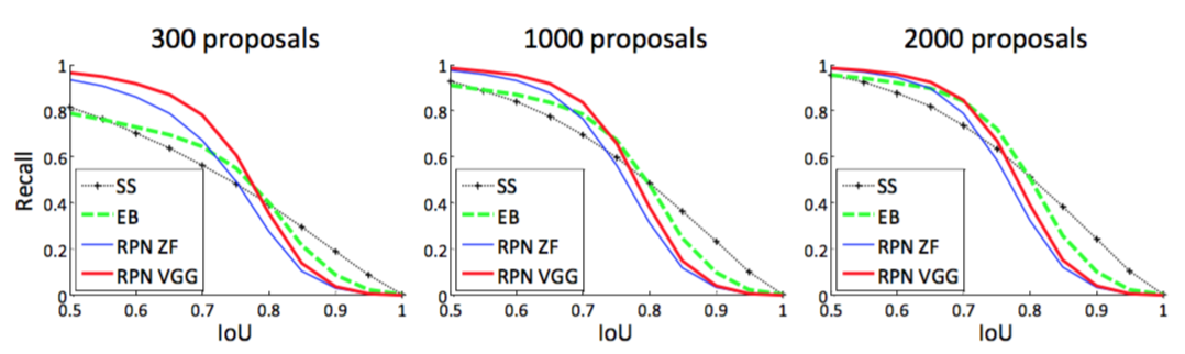
Figure 4: Recall vs. IoU overlap ratio on the PASCAL VOC 2007 test set.

在图4中，我们显示了使用300，1000和2000个提议的结果。我们与SS和EB进行比较，根据这些方法产生的置信度，N个提议是排名前N的提议。从图中可以看出，当提议数量从2000个减少到300个时，RPN方法表现优雅。这就解释了为什么RPN在使用300个提议时具有良好的最终检测mAP。正如我们之前分析过的，这个属性主要归因于RPN的cls项。当提议较少时，SS和EB的召回率下降的比RPN更快。

图4：PASCAL VOC 2007测试集上的召回率和IoU重叠率。

One-Stage Detection vs. Two-Stage Proposal + Detection. The OverFeat paper [9] proposes a detection method that uses regressors and classifiers on sliding windows over convolutional feature maps. OverFeat is a one-stage, class-specific detection pipeline, and ours is a two-stage cascade consisting of class-agnostic proposals and class-specific detections. In OverFeat, the region-wise features come from a sliding window of one aspect ratio over a scale pyramid. These features are used to simultaneously determine the location and category of objects. In RPN, the features are from square ($3\times 3$) sliding windows and predict proposals relative to anchors with different scales and aspect ratios. Though both methods use sliding windows, the region proposal task is only the first stage of Faster R-CNN —— the downstream Fast R-CNN detector attends to the proposals to refine them. In the second stage of our cascade, the region-wise features are adaptively pooled [1], [2] from proposal boxes that more faithfully cover the features of the regions. We believe these features lead to more accurate detections.

一阶段检测与两阶段提议+检测。OverFeat论文[9]提出了一种在卷积特征映射的滑动窗口上使用回归器和分类器的检测方法。OverFeat是一个一阶段，类别特定的检测流程，而我们的是两阶段级联，包括类不可知的提议和类别特定的检测。在OverFeat中，区域特征来自一个尺度金字塔上一个长宽比的滑动窗口。这些特征用于同时确定目标的位置和类别。在RPN中，这些特征来自正方形（$3\times 3$）滑动窗口，并且预测相对于锚点具有不同尺度和长宽比的提议。虽然这两种方法都使用滑动窗口，但区域提议任务只是Faster R-CNN的第一阶段——下游的Fast R-CNN检测器会致力于对提议进行细化。在我们级联的第二阶段，在更忠实覆盖区域特征的提议框中，区域特征自适应地聚集[1]，[2]。我们相信这些功能会带来更准确的检测结果。

To compare the one-stage and two-stage systems, we emulate the OverFeat system (and thus also circumvent other differences of implementation details) by one-stage Fast R-CNN. In this system, the “proposals” are dense sliding windows of 3 scales (128, 256, 512) and 3 aspect ratios (1:1, 1:2, 2:1). Fast R-CNN is trained to predict class-specific scores and regress box locations from these sliding windows. Because the OverFeat system adopts an image pyramid, we also evaluate using convolutional features extracted from 5 scales. We use those 5 scales as in [1], [2].

为了比较一阶段和两阶段系统，我们通过一阶段Fast R-CNN来模拟OverFeat系统（从而也规避了实现细节的其他差异）。在这个系统中，“提议”是3个尺度（128，256，512）和3个长宽比（1:1，1:2，2:1）的密集滑动窗口。训练Fast R-CNN来预测类别特定的分数，并从这些滑动窗口中回归边界框位置。由于OverFeat系统采用图像金字塔，我们也使用从5个尺度中提取的卷积特征进行评估。我们使用[1]，[2]中5个尺度。

Table 10 compares the two-stage system and two variants of the one-stage system. Using the ZF model, the one-stage system has an mAP of $53.9\%$. This is lower than the two-stage system ($58.7\%$) by $4.8\%$. This experiment justifies the effectiveness of cascaded region proposals and object detection. Similar observations are reported in [2], [39], where replacing SS region proposals with sliding windows leads to $\sim 6\%$ degradation in both papers. We also note that the one-stage system is slower as it has considerably more proposals to process.

Table 10: One-Stage Detection vs. Two-Stage Proposal + Detection. Detection results are on the PASCAL VOC 2007 test set using the ZF model and Fast R-CNN. RPN uses unshared features.

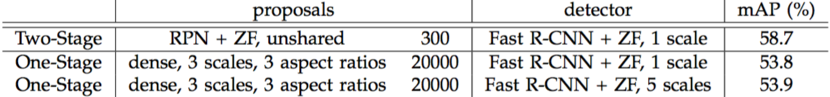
表10比较了两阶段系统和一阶段系统的两个变种。使用ZF模型，一阶段系统具有$53.9\%$的mAP。这比两阶段系统（$58.7\%$）低$4.8\%$。这个实验验证了级联区域提议和目标检测的有效性。在文献[2]，[39]中报道了类似的观察结果，在这两篇论文中，用滑动窗取代SS区域提议会导致$\sim 6\%$的退化。我们也注意到，一阶段系统更慢，因为它产生了更多的提议。

表10：一阶段检测与两阶段提议+检测。使用ZF模型和Fast R-CNN在PASCAL VOC 2007测试集上的检测结果。RPN使用未共享的功能。

4.2 Experiments on MS COCO

We present more results on the Microsoft COCO object detection dataset [12]. This dataset involves 80 object categories. We experiment with the 80k images on the training set, 40k images on the validation set, and 20k images on the test-dev set. We evaluate the mAP averaged for $IoU \in [0.5:0.05:0.95]$ (COCO’s standard metric, simply denoted as mAP@[.5, .95]) and mAP@0.5 (PASCAL VOC’s metric).

4.2 在MS COCO上的实验

我们在Microsoft COCO目标检测数据集[12]上提供了更多的结果。这个数据集包含80个目标类别。我们用训练集上的8万张图像，验证集上的4万张图像以及测试开发集上的2万张图像进行实验。我们评估了$IoU \in [0.5:0.05:0.95]$的平均mAP（COCO标准度量，简称为mAP@[.5,.95]）和mAP@0.5（PASCAL VOC度量）。

There are a few minor changes of our system made for this dataset. We train our models on an 8-GPU implementation, and the effective mini-batch size becomes 8 for RPN (1 per GPU) and 16 for Fast R-CNN (2 per GPU). The RPN step and Fast R-CNN step are both trained for 240k iterations with a learning rate of 0.003 and then for 80k iterations with 0.0003. We modify the learning rates (starting with 0.003 instead of 0.001) because the mini-batch size is changed. For the anchors, we use 3 aspect ratios and 4 scales (adding $64^2$), mainly motivated by handling small objects on this dataset. In addition, in our Fast R-CNN step, the negative samples are defined as those with a maximum IoU with ground truth in the interval of [0,0.5), instead of [0.1,0.5) used in [1], [2]. We note that in the SPPnet system [1], the negative samples in [0.1, 0.5) are used for network fine-tuning, but the negative samples in [0, 0.5) are still visited in the SVM step with hard-negative mining. But the Fast R-CNN system [2] abandons the SVM step, so the negative samples in [0,0.1) are never visited. Including these [0,0.1) samples improves mAP@0.5 on the COCO dataset for both Fast R-CNN and Faster R-CNN systems (but the impact is negligible on PASCAL VOC).

我们的系统对这个数据集做了一些小的改动。我们在8 GPU实现上训练我们的模型，RPN（每个GPU 1个）和Fast R-CNN（每个GPU 2个）的有效最小批大小为8个。RPN步骤和Fast R-CNN步骤都以24万次迭代进行训练，学习率为0.003，然后以0.0003的学习率进行8万次迭代。我们修改了学习率（从0.003而不是0.001开始），因为小批量数据的大小发生了变化。对于锚点，我们使用3个长宽比和4个尺度（加上$64^2$），这主要是通过处理这个数据集上的小目标来激发的。此外，在我们的Fast R-CNN步骤中，负样本定义为与实际边界框的最大IOU在[0，0.5)区间内的样本，而不是[1]，[2]中使用的[0.1,0.5)之间。我们注意到，在SPPnet系统[1]中，在[0.1，0.5)中的负样本用于网络微调，但[0,0.5)中的负样本仍然在具有难例挖掘SVM步骤中被访问。但是Fast R-CNN系统[2]放弃了SVM步骤，所以[0,0.1]中的负样本都不会被访问。包括这些[0,0.1)的样本，在Fast R-CNN和Faster R-CNN系统在COCO数据集上改进了mAP@0.5（但对PASCAL VOC的影响可以忽略不计）。

The rest of the implementation details are the same as on PASCAL VOC. In particular, we keep using 300 proposals and single-scale ($s=600$) testing. The testing time is still about 200ms per image on the COCO dataset.

其余的实现细节与PASCAL VOC相同。特别的是，我们继续使用300个提议和单一尺度（$s=600$）测试。COCO数据集上的测试时间仍然是大约200ms处理一张图像。

In Table 11 we first report the results of the Fast R-CNN system [2] using the implementation in this paper. Our Fast R-CNN baseline has $39.3\%$ mAP@0.5 on the test-dev set, higher than that reported in [2]. We conjecture that the reason for this gap is mainly due to the definition of the negative samples and also the changes of the mini-batch sizes. We also note that the mAP@[.5, .95] is just comparable.

Table 11: Object detection results (%) on the MS COCO dataset. The model is VGG-16.

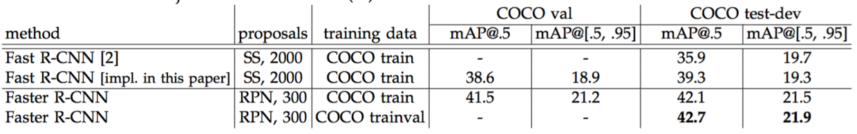
在表11中，我们首先报告了使用本文实现的Fast R-CNN系统[2]的结果。我们的Fast R-CNN基准在test-dev数据集上有$39.3\%$的mAP@0.5，比[2]中报告的更高。我们推测造成这种差距的原因主要是由于负样本的定义以及小批量大小的变化。我们也注意到mAP@[.5，.95]恰好相当。

表11：在MS COCO数据集上的目标检测结果(%)。模型是VGG-16。

Next we evaluate our Faster R-CNN system. Using the COCO training set to train, Faster R-CNN has $42.1\%$ mAP@0.5 and $21.5\%$ mAP@[.5, .95] on the COCO test-dev set. This is $2.8\%$ higher for mAP@0.5 and $2.2\%$ higher for mAP@[.5, .95] than the Fast R-CNN counterpart under the same protocol (Table 11). This indicates that RPN performs excellent for improving the localization accuracy at higher IoU thresholds. Using the COCO trainval set to train, Faster R-CNN has $42.7\%$ mAP@0.5 and $21.9\%$ mAP@[.5, .95] on the COCO test-dev set. Figure 6 shows some results on the MS COCO test-dev set.

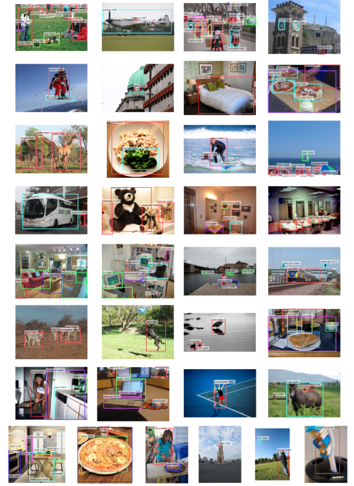
Figure 6: Selected examples of object detection results on the MS COCO test-dev set using the Faster R-CNN system. The model is VGG-16 and the training data is COCO trainval ($42.7\%$ mAP@0.5 on the test-dev set). Each output box is associated with a category label and a softmax score in [0, 1]. A score threshold of 0.6 is used to display these images. For each image, one color represents one object category in that image.

接下来我们评估我们的Faster R-CNN系统。使用COCO训练集训练，在COCO测试开发集上Faster R-CNNN有$42.1\%$的mAP@0.5和$21.5\%$的mAP@[0.5，0.95]。与相同协议下的Fast R-CNN相比，mAP@0.5要高$2.8\%$，mAP@[.5, .95]要高$2.2\%$（表11）。这表明，在更高的IoU阈值上，RPN对提高定位精度表现出色。使用COCO训练集训练，在COCO测试开发集上Faster R-CNN有$42.7\%$的mAP@0.5和$21.9\%$的mAP@[.5, .95]。图6显示了MS COCO测试开发数据集中的一些结果。

图6：使用Faster R-CNN系统在MS COCO test-dev数据集上选择的目标检测结果示例。该模型是VGG-16，训练数据是COCO训练数据（在测试开发数据集上为$42.7\%$的mAP@0.5）。每个输出框都与一个类别标签和[0, 1]之间的softmax分数相关联。使用0.6的分数阈值来显示这些图像。对于每张图像，一种颜色表示该图像中的一个目标类别。

Faster R-CNN in ILSVRC & COCO 2015 competitions. We have demonstrated that Faster R-CNN benefits more from better features, thanks to the fact that the RPN completely learns to propose regions by neural networks. This observation is still valid even when one increases the depth substantially to over 100 layers [18]. Only by replacing VGG-16 with a 101-layer residual net (ResNet-101) [18], the Faster R-CNN system increases the mAP from $41.5
%/21.2\%$ (VGG-16) to $48.4\%/27.2\%$ (ResNet-101) on the COCO val set. With other improvements orthogonal to Faster R-CNN, He et al. [18] obtained a single-model result of $55.7\%/34.9\%$ and an ensemble result of $59.0\%/37.4\%$ on the COCO test-dev set, which won the 1st place in the COCO 2015 object detection competition. The same system [18] also won the 1st place in the ILSVRC 2015 object detection competition, surpassing the second place by absolute $8.5\%$. RPN is also a building block of the 1st-place winning entries in ILSVRC 2015 localization and COCO 2015 segmentation competitions, for which the details are available in [18] and [15] respectively.

在ILSVRC和COCO 2015比赛中的Faster R-CNN。我们已经证明，由于RPN通过神经网络完全学习了提议区域，Faster R-CNN从更好的特征中受益更多。即使将深度增加到100层以上，这种观察仍然是有效的[18]。仅用101层残差网络（ResNet-101）代替VGG-16，Faster R-CNN系统就将mAP从$41.5
%/21.2\%$（VGG-16）增加到$48.4\%/27.2\%$（ResNet-101）。与其他改进正交于Faster R-CNN，何等人[18]在COCO测试开发数据集上获得了单模型$55.7\%/34.9\%$的结果和$59.0\%/37.4\%$的组合结果，在COCO 2015目标检测竞赛中获得了第一名。同样的系统[18]也在ILSVRC 2015目标检测竞赛中获得了第一名，超过第二名绝对的$8.5\%$。RPN也是ILSVRC2015定位和COCO2015分割竞赛第一名获奖输入的基石，详情请分别参见[18]和[15]。

4.3 From MS COCO to PASCAL VOC

Large-scale data is of crucial importance for improving deep neural networks. Next, we investigate how the MS COCO dataset can help with the detection performance on PASCAL VOC.

4.3 从MS COCO到PASCAL VOC

大规模数据对改善深度神经网络至关重要。接下来，我们调查MS COCO数据集如何帮助改进在PASCAL VOC上的检测性能。

As a simple baseline, we directly evaluate the COCO detection model on the PASCAL VOC dataset, without fine-tuning on any PASCAL VOC data. This evaluation is possible because the categories on COCO are a superset of those on PASCAL VOC. The categories that are exclusive on COCO are ignored in this experiment, and the softmax layer is performed only on the 20 categories plus background. The mAP under this setting is $76.1\%$ on the PASCAL VOC 2007 test set (Table 12). This result is better than that trained on VOC07+12 ($73.2\%$) by a good margin, even though the PASCAL VOC data are not exploited.

作为一个简单的基准数据，我们直接在PASCAL VOC数据集上评估COCO检测模型，而无需在任何PASCAL VOC数据上进行微调。这种评估是可能的，因为COCO类别是PASCAL VOC上类别的超集。在这个实验中忽略COCO专有的类别，softmax层仅在20个类别和背景上执行。这种设置下PASCAL VOC 2007测试集上的mAP为$76.1\%$（表12）。即使没有利用PASCAL VOC的数据，这个结果也好于在VOC07+12($73.2\%$)上训练的模型的结果。

Then we fine-tune the COCO detection model on the VOC dataset. In this experiment, the COCO model is in place of the ImageNet-pre-trained model (that is used to initialize the network weights), and the Faster R-CNN system is fine-tuned as described in Section 3.2. Doing so leads to $78.8\%$ mAP on the PASCAL VOC 2007 test set. The extra data from the COCO set increases the mAP by $5.6\%$. Table 6 shows that the model trained on COCO+VOC has the best AP for every individual category on PASCAL VOC 2007. Similar improvements are observed on the PASCAL VOC 2012 test set (Table 12 and Table 7). We note that the test-time speed of obtaining these strong results is still about 200ms per image.

Table 6: Results on PASCAL VOC 2007 test set with Fast R-CNN detectors and VGG-16. For RPN, the train-time proposals for Fast R-CNN are 2000. $RPN^*$ denotes the unsharing feature version.

Table 12: Detection mAP (%) of Faster R-CNN on PASCAL VOC 2007 test set and 2012 test set using different training data. The model is VGG-16. “COCO” denotes that the COCO trainval set is used for training. See also Table 6 and Table 7.

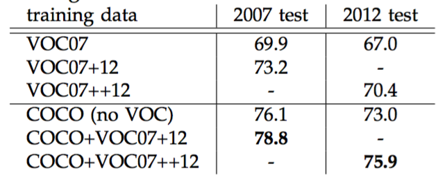
Table 7: Results on PASCAL VOC 2012 test set with Fast R-CNN detectors and VGG-16. For RPN, the train-time proposals for Fast R-CNN are 2000.

然后我们在VOC数据集上对COCO检测模型进行微调。在这个实验中，COCO模型代替了ImageNet的预训练模型（用于初始化网络权重），Faster R-CNN系统按3.2节所述进行微调。这样做在PASCAL VOC 2007测试集上可以达到$78.8\%$的mAP。来自COCO集合的额外数据增加了$5.6\%$的mAP。表6显示，在PASCAL VOC 2007上，使用COCO+VOC训练的模型在每个类别上具有最好的AP值。在PASCAL VOC 2012测试集（表12和表7）中也观察到类似的改进。我们注意到获得这些强大结果的测试时间速度仍然是每张图像200ms左右。

表6：Fast R-CNN检测器和VGG-16在PASCAL VOC 2007测试集上的结果。对于RPN，Fast R-CNN的训练时的提议数量是2000。$RPN^*$表示取消共享特征的版本。

表12：使用不同的训练数据在PASCAL VOC 2007测试集和2012测试集上检测Faster R-CNN的检测mAP（％）。模型是VGG-16。“COCO”表示COCOtrainval数据集用于训练。另见表6和表7。

表7：Fast R-CNN检测器和VGG-16在PASCAL VOC 2012测试集上的结果。对于RPN，Fast R-CNN训练时的提议数量为2000。

5. CONCLUSION

We have presented RPNs for efficient and accurate region proposal generation. By sharing convolutional features with the down-stream detection network, the region proposal step is nearly cost-free. Our method enables a unified, deep-learning-based object detection system to run at near real-time frame rates. The learned RPN also improves region proposal quality and thus the overall object detection accuracy.

5. 结论

我们已经提出了RPN来生成高效，准确的区域提议。通过与下游检测网络共享卷积特征，区域提议步骤几乎是零成本的。我们的方法使统一的，基于深度学习的目标检测系统能够以接近实时的帧率运行。学习到的RPN也提高了区域提议的质量，从而提高了整体的目标检测精度。

REFERENCES

[1] K. He, X. Zhang, S. Ren, and J. Sun, “Spatial pyramid pooling in deep convolutional networks for visual recognition,” in European Conference on Computer Vision (ECCV), 2014.

[2] R. Girshick, “Fast R-CNN,” in IEEE International Conference on Computer Vision (ICCV), 2015.

[3] K. Simonyan and A. Zisserman, “Very deep convolutional networks for large-scale image recognition,” in International Conference on Learning Representations (ICLR), 2015.

[4] J. R. Uijlings, K. E. van de Sande, T. Gevers, and A. W. Smeulders, “Selective search for object recognition,” International
Journal of Computer Vision (IJCV), 2013.

[5] R. Girshick, J. Donahue, T. Darrell, and J. Malik, “Rich feature hierarchies for accurate object detection and semantic segmentation,” in IEEE Conference on Computer Vision and Pattern Recognition (CVPR), 2014.

[6] C. L. Zitnick and P. Dollár, “Edge boxes: Locating object proposals from edges,” in European Conference on Computer Vision(ECCV),2014.

[7] J. Long, E. Shelhamer, and T. Darrell, “Fully convolutional networks for semantic segmentation,” in IEEE Conference on Computer Vision and Pattern Recognition (CVPR), 2015.

[8] P. F. Felzenszwalb, R. B. Girshick, D. McAllester, and D. Ramanan, “Object detection with discriminatively trained part-based models,” IEEE Transactions on Pattern Analysis and Machine Intelligence (TPAMI), 2010.

[9] P. Sermanet, D. Eigen, X. Zhang, M. Mathieu, R. Fergus, and Y. LeCun, “Overfeat: Integrated recognition, localization and detection using convolutional networks,” in International Conference on Learning Representations (ICLR), 2014.

[10] S. Ren, K. He, R. Girshick, and J. Sun, “FasterR-CNN: Towards real-time object detection with region proposal networks,” in
Neural Information Processing Systems (NIPS), 2015.

[11] M. Everingham, L. Van Gool, C. K. I. Williams, J. Winn, and A. Zisserman, “The PASCAL Visual Object Classes Challenge 2007 (VOC2007) Results,” 2007.

[12] T.-Y. Lin, M. Maire, S. Belongie, J. Hays, P. Perona, D. Ramanan, P. Dollár, and C. L. Zitnick, “Microsoft COCO: Common Objects in Context,” in European Conference on Computer Vision (ECCV), 2014.

[13] S. Song and J. Xiao, “Deep sliding shapes for amodal 3d object detection in rgb-d images,” arXiv:1511.02300, 2015.

[14] J. Zhu, X. Chen, and A. L. Yuille, “DeePM: A deep part-based model for object detection and semantic part localization,” arXiv:1511.07131, 2015.

[15] J. Dai, K. He, and J. Sun, “Instance-aware semantic segmentation via multi-task network cascades,” arXiv:1512.04412, 2015.

[16] J. Johnson, A. Karpathy, and L. Fei-Fei, “Densecap: Fully convolutional localization networks for dense captioning,” arXiv:1511.07571, 2015.

[17] D. Kislyuk, Y. Liu, D. Liu, E. Tzeng, and Y. Jing, “Human curation and convnets: Powering item-to-item recommendations on pinterest,” arXiv:1511.04003, 2015.

[18] K. He, X. Zhang, S. Ren, and J. Sun, “Deep residual learning for image recognition,” arXiv:1512.03385, 2015.

[19] J. Hosang, R. Benenson, and B. Schiele, “How good are detection proposals, really?” in British Machine Vision Conference (BMVC), 2014.

[20] J. Hosang, R. Benenson, P. Dollar, and B. Schiele, “What makes for effective detection proposals?” IEEE Transactions on Pattern Analysis and Machine Intelligence (TPAMI), 2015.

[21] N. Chavali, H. Agrawal, A. Mahendru, and D. Batra, “Object-Proposal Evaluation Protocol is ’Gameable’,” arXiv: 1505.05836, 2015.

[22] J. Carreira and C. Sminchisescu, “CPMC: Automatic object segmentation using constrained parametric min-cuts,” IEEE Transactions on Pattern Analysis and Machine Intelligence (TPAMI), 2012.

[23] P. Arbelaez, J. Pont-Tuset, J. T. Barron, F. Marques, and J. Malik, “Multiscale combinatorial grouping,” in IEEE Conference on Computer Vision and Pattern Recognition (CVPR), 2014.

[24] B. Alexe, T. Deselaers, and V. Ferrari, “Measuring the objectness of image windows,” IEEE Transactions on Pattern Analysis and Machine Intelligence (TPAMI), 2012.

[25] C. Szegedy, A. Toshev, and D. Erhan, “Deep neural networks for object detection,” in Neural Information Processing Systems (NIPS), 2013.

[26] D. Erhan, C. Szegedy, A. Toshev, and D. Anguelov, “Scalable object detection using deep neural networks,” in IEEE Conference on Computer Vision and Pattern Recognition (CVPR), 2014.

[27] C. Szegedy, S. Reed, D. Erhan, and D. Anguelov, “Scalable, high-quality object detection,” arXiv:1412.1441 (v1), 2015.

[28] P. O. Pinheiro, R. Collobert, and P. Dollar, “Learning to segment object candidates,” in Neural Information Processing Systems (NIPS), 2015.

[29] J. Dai, K. He, and J. Sun, “Convolutional feature masking for joint object and stuff segmentation,” in IEEE Conference on Computer Vision and Pattern Recognition (CVPR), 2015.

[30] S. Ren, K. He, R. Girshick, X. Zhang, and J. Sun, “Object detection networks on convolutional feature maps,” arXiv:1504.06066, 2015.

[31] J. K. Chorowski, D. Bahdanau, D. Serdyuk, K. Cho, and Y. Bengio, “Attention-based models for speech recognition,” in Neural Information Processing Systems (NIPS), 2015.

[32] M. D. Zeiler and R. Fergus, “Visualizing and understanding convolutional neural networks,” in European Conference on Computer Vision (ECCV), 2014.

[33] V. Nair and G. E. Hinton, “Rectified linear units improve restricted boltzmann machines,” in International Conference on Machine Learning (ICML), 2010.

[34] C. Szegedy, W. Liu, Y. Jia, P. Sermanet, S. Reed, D. Anguelov, D. Erhan, and A. Rabinovich, “Going deeper with convolutions,” in IEEE Conference on Computer Vision and Pattern Recognition (CVPR), 2015.

[35] Y. LeCun, B. Boser, J. S. Denker, D. Henderson, R. E. Howard, W. Hubbard, and L. D. Jackel, “Backpropagation applied to handwritten zip code recognition,” Neural computation, 1989.

[36] O. Russakovsky, J. Deng, H. Su, J. Krause, S. Satheesh, S. Ma, Z. Huang, A. Karpathy, A. Khosla, M. Bernstein, A. C. Berg, and L. Fei-Fei, “ImageNet Large Scale Visual Recognition Challenge,” in International Journal of Computer Vision (IJCV), 2015.

[37] A. Krizhevsky, I. Sutskever, and G. Hinton, “Imagenet classification with deep convolutional neural networks,” in Neural Information Processing Systems (NIPS), 2012.

[38] Y. Jia, E. Shelhamer, J. Donahue, S. Karayev, J. Long, R. Girshick, S. Guadarrama, and T. Darrell, “Caffe: Convolutional architecture for fast feature embedding,” arXiv:1408.5093, 2014.

[39] K. Lenc and A. Vedaldi, “R-CNN minus R,” in British Machine Vision Conference (BMVC), 2015.