文章作者:Tyan
博客:noahsnail.com | CSDN | 简书
声明:作者翻译论文仅为学习,如有侵权请联系作者删除博文,谢谢!
翻译论文汇总:https://github.com/SnailTyan/deep-learning-papers-translation
R-FCN: Object Detection via Region-based Fully Convolutional Networks
Abstract
We present region-based, fully convolutional networks for accurate and efficient object detection. In contrast to previous region-based detectors such as Fast/Faster R-CNN [6, 18] that apply a costly per-region subnetwork hundreds of times, our region-based detector is fully convolutional with almost all computation shared on the entire image. To achieve this goal, we propose position-sensitive score maps to address a dilemma between translation-invariance in image classification and translation-variance in object detection. Our method can thus naturally adopt fully convolutional image classifier backbones, such as the latest Residual Networks (ResNets) [9], for object detection. We show competitive results on the PASCAL VOC datasets (e.g., $83.6\%$ mAP on the 2007 set) with the 101-layer ResNet. Meanwhile, our result is achieved at a test-time speed of 170ms per image, 2.5-20× faster than the Faster R-CNN counterpart. Code is made publicly available at: https://github.com/daijifeng001/r-fcn.
摘要
我们提出了基于区域的全卷积网络,以实现准确和高效的目标检测。与先前的基于区域的检测器(如Fast/Faster R-CNN [6,18])相比,这些检测器应用昂贵的每个区域子网络数百次,我们的基于区域的检测器是全卷积的,几乎所有计算都在整张图像上共享。为了实现这一目标,我们提出了位置敏感分数图,以解决图像分类中的平移不变性与目标检测中的平移变化之间的困境。因此,我们的方法可以自然地采用全卷积图像分类器的主干网络,如最新的残差网络(ResNets)[9],用于目标检测。我们使用101层ResNet在PASCAL VOC数据集上展示了具有竞争力的结果(例如,2007数据集上$83.6\%$的mAP)。同时,我们的测试结果是以每张图像170ms的测试速度实现的,比Faster R-CNN对应部分速度快2.5-20倍。代码公开发布在:[https://github.com/daijifeng001/r-fcn](https://github.com/daijifeng001/r-fcn)。
1. Introduction
A prevalent family [8, 6, 18] of deep networks for object detection can be divided into two subnetworks by the Region-of-Interest (RoI) pooling layer [6]: (i) a shared, “fully convolutional” subnetwork independent of RoIs, and (ii) an RoI-wise subnetwork that does not share computation. This decomposition [8] was historically resulted from the pioneering classification architectures, such as AlexNet [10] and VGG Nets [23], that consist of two subnetworks by design —— a convolutional subnetwork ending with a spatial pooling layer, followed by several fully-connected (fc) layers. Thus the (last) spatial pooling layer in image classification networks is naturally turned into the RoI pooling layer in object detection networks [8, 6, 18].
1. 引言
流行的目标检测深度网络家族[8,6,18]通过感兴趣区域(RoI)池化层[6]可以划分成两个子网络:(1)独立于RoI的共享“全卷积”子网络,(ii)不共享计算的RoI子网络。这种分解[8]以往是由开创性的分类架构产生的,例如AlexNet[10]和VGG Nets[23]等,在设计上它由两个子网络组成——一个卷积子网络以空间池化层结束,后面是几个全连接(fc)层。因此,图像分类网络中的(最后一个)空间池化层在目标检测网络中[8,6,18]自然地变成了RoI池化层。
But recent state-of-the-art image classification networks such as Residual Nets (ResNets) [9] and GoogLeNets [24, 26] are by design fully convolutional. By analogy, it appears natural to use all convolutional layers to construct the shared, convolutional subnetwork in the object detection architecture, leaving the RoI-wise subnetwork no hidden layer. However, as empirically investigated in this work, this naïve solution turns out to have considerably inferior detection accuracy that does not match the network’s superior classification accuracy. To remedy this issue, in the ResNet paper [9] the RoI pooling layer of the Faster R-CNN detector [18] is unnaturally inserted between two sets of convolutional layers —— this creates a deeper RoI-wise subnetwork that improves accuracy, at the cost of lower speed due to the unshared per-RoI computation.
但是最近最先进的图像分类网络,如ResNet(ResNets)[9]和GoogLeNets[24,26]是全卷积的。通过类比,在目标检测架构中使用所有卷积层来构建共享的卷积子网络似乎是很自然的,使得RoI的子网络没有隐藏层。然而,在这项工作中通过经验性的调查发现,这个天真的解决方案有相当差的检测精度,不符合网络的优秀分类精度。为了解决这个问题,在ResNet论文[9]中,Faster R-CNN检测器[18]的RoI池层不自然地插入在两组卷积层之间——这创建了更深的RoI子网络,其改善了精度,由于非共享的RoI计算,因此是以更低的速度为代价。
We argue that the aforementioned unnatural design is caused by a dilemma of increasing translation invariance for image classification vs. respecting translation variance for object detection. On one hand, the image-level classification task favors translation invariance —— shift of an object inside an image should be indiscriminative. Thus, deep (fully) convolutional architectures that are as translation-invariant as possible are preferable as evidenced by the leading results on ImageNet classification [9, 24, 26]. On the other hand, the object detection task needs localization representations that are translation-variant to an extent. For example, translation of an object inside a candidate box should produce meaningful responses for describing how good the candidate box overlaps the object. We hypothesize that deeper convolutional layers in an image classification network are less sensitive to translation. To address this dilemma, the ResNet paper’s detection pipeline [9] inserts the RoI pooling layer into convolutions —— this region-specific operation breaks down translation invariance, and the post-RoI convolutional layers are no longer translation-invariant when evaluated across different regions. However, this design sacrifices training and testing efficiency since it introduces a considerable number of region-wise layers (Table 1).
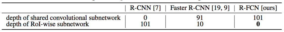
Table 1: Methodologies of region-based detectors using ResNet-101 [9].
我们认为,前述的非自然设计是由于增加图像分类的变换不变性与目标检测的平移可变性而导致的两难境地。一方面,图像级别的分类任务有利于平移不变性——图像内目标的移动应该是无差别的。因此,深度(全)卷积架构尽可能保持平移不变,这一点可以从ImageNet分类[9,24,26]的主要结果中得到证实。另一方面,目标检测任务的定位表示需要一定程度上的平移可变性。例如,在候选框内目标变换应该产生有意义的响应,用于描述候选框与目标的重叠程度。我们假设图像分类网络中较深的卷积层对平移不太敏感。为了解决这个困境,ResNet论文的检测流程[9]将RoI池化层插入到卷积中——特定区域的操作打破了平移不变性,当在不同区域进行评估时,RoI后卷积层不再是平移不变的。然而,这个设计牺牲了训练和测试效率,因为它引入了大量的区域层(表1)。
表1:使用ResNet-101的基于区域的检测器方法[9]。
In this paper, we develop a framework called Region-based Fully Convolutional Network (R-FCN) for object detection. Our network consists of shared, fully convolutional architectures as is the case of FCN [15]. To incorporate translation variance into FCN, we construct a set of position-sensitive score maps by using a bank of specialized convolutional layers as the FCN output. Each of these score maps encodes the position information with respect to a relative spatial position (e.g., “to the left of an object”). On top of this FCN, we append a position-sensitive RoI pooling layer that shepherds information from these score maps, with no weight (convolutional/fc) layers following. The entire architecture is learned end-to-end. All learnable layers are convolutional and shared on the entire image, yet encode spatial information required for object detection. Figure 1 illustrates the key idea and Table 1 compares the methodologies among region-based detectors.
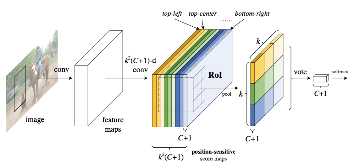
Figure 1: Key idea of R-FCN for object detection. In this illustration, there are k × k = 3 × 3 position-sensitive score maps generated by a fully convolutional network. For each of the k × k bins in an RoI, pooling is only performed on one of the $k^2$ maps (marked by different colors).
在本文中,我们开发了一个称为基于区域的全卷积网络(R-FCN)框架来进行目标检测。我们的网络由共享的全卷积架构组成,就像FCN[15]一样。为了将平移可变性并入FCN,我们通过使用一组专门的卷积层作为FCN输出来构建一组位置敏感的分数图。这些分数图中的每一个都对关于相对空间位置(的位置信息进行编码例如,“在目标的左边”)。在这个FCN之上,我们添加了一个位置敏感的RoI池化层,它从这些分数图中获取信息,并且后面没有权重(卷积/fc)层。整个架构是端到端的学习。所有可学习的层都是卷积的,并在整个图像上共享,但对目标检测所需的空间信息进行编码。图1说明了关键思想,表1比较了基于区域的检测器方法。
图1:R-FCN目标检测的主要思想。在这个例子中,由全卷积网络生成了k×k=3×3的位置敏感分数图。对于RoI中的每个k×k组块,仅在$k^2$个映射中的一个上执行池化(用不同的颜色标记)。
Using the 101-layer Residual Net (ResNet-101) [9] as the backbone, our R-FCN yields competitive results of $83.6\%$ mAP on the PASCAL VOC 2007 set and $82.0\%$ the 2012 set. Meanwhile, our results are achieved at a test-time speed of 170ms per image using ResNet-101, which is 2.5× to 20× faster than the Faster R-CNN + ResNet-101 counterpart in [9]. These experiments demonstrate that our method manages to address the dilemma between invariance/variance on translation, and fully convolutional image-level classifiers such as ResNets can be effectively converted to fully convolutional object detectors. Code is made publicly available at: https://github.com/daijifeng001/r-fcn.
使用101层残余网络(ResNet-101)[9]作为主干网络,我们的R-FCN在PASCAL VOC 2007数据集和2012数据集上分别获得了$83.6\%$ mAP和 $82.0\%$ mAP。同时,使用ResNet-101,我们的结果在测试时是以每张图像170ms的速度实现的,比[9]中对应的Faster R-CNN + ResNet-101快了2.5倍到20倍。这些实验表明,我们的方法设法解决平移不变性/可变性和全卷积图像级分类器之间的困境,如ResNet可以有效地转换为全卷积目标检测器。代码公开发布在:https://github.com/daijifeng001/r-fcn。
2. Our approach
Overview. Following R-CNN [7], we adopt the popular two-stage object detection strategy [7, 8, 6, 18, 1, 22] that consists of: (i) region proposal, and (ii) region classification. Although methods that do not rely on region proposal do exist (e.g., [17, 14]), region-based systems still possess leading accuracy on several benchmarks [5, 13, 20]. We extract candidate regions by the Region Proposal Network (RPN) [18], which is a fully convolutional architecture in itself. Following [18], we share the features between RPN and R-FCN. Figure 2 shows an overview of the system.
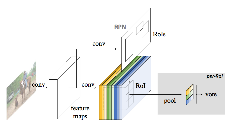
Figure 2: Overall architecture of R-FCN. A Region Proposal Network (RPN) [18] proposes candidate RoIs, which are then applied on the score maps. All learnable weight layers are convolutional and are computed on the entire image; the per-RoI computational cost is negligible.
2. 我们的方法
概述。根据R-CNN[7],我们采用了流行的两阶段目标检测策略[7,8,6,18,1,22],其中包括:(i)区域提议和(ii)区域分类。尽管不依赖区域提议的方法确实存在(例如,[17,14]),但是基于区域的系统在几个基准数据集中仍然具有领先的准确性[5,13,20]。我们通过区域提议网络(RPN)提取候选区域[18],其本身就是一个全卷积架构。在[18]之后,我们在RPN和R-FCN之间的共享特征。图2显示了系统的概述。
图2:R-FCN的总体架构。区域建议网络(RPN)[18]提出了候选RoI,然后将其应用于评分图上。所有可学习的权重层都是卷积的,并在整个图像上计算;每个RoI的计算成本可以忽略不计。
Given the proposal regions (RoIs), the R-FCN architecture is designed to classify the RoIs into object categories and background. In R-FCN, all learnable weight layers are convolutional and are computed on the entire image. The last convolutional layer produces a bank of $k^2$ position-sensitive score maps for each category, and thus has a $k^2(C+1)$-channel output layer with $C$ object categories ($+1$ for background). The bank of $k^2$ score maps correspond to a $k\times k$ spatial grid describing relative positions. For example, with $k\times k = 3\times 3$, the 9 score maps encode the cases of {top-left, top-center, top-right, …, bottom-right} of an object category.
鉴于提议区域(RoI),R-FCN架构被设计成将RoI分类为目标类别和背景。在R-FCN中,所有可学习的权重层都是卷积的,并在整个图像上进行计算。最后一个卷积层为每个类别产生一堆大小为$k^2$的位置敏感分数图,从而得到一个具有$C$个目标类别的$k^2(C+1)$通道输出层($+1$为背景)。一堆$k^2$个分数图对应于描述相对位置的$k\times k$空间网格。例如,对于$k\times k = 3\times 3$,大小为9的分数图编码目标类别在{左上,右上,右上,…,右下}的情况。
R-FCN ends with a position-sensitive RoI pooling layer. This layer aggregates the outputs of the last convolutional layer and generates scores for each RoI. Unlike [8, 6], our position-sensitive RoI layer conducts selective pooling, and each of the $k\times k$ bin aggregates responses from only one score map out of the bank of $k\times k$ score maps. With end-to-end training, this RoI layer shepherds the last convolutional layer to learn specialized position-sensitive score maps. Figure 1 illustrates this idea. Figure 3 and 4 visualize an example. The details are introduced as follows.
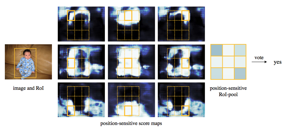
Figure 3: Visualization of R-FCN (k × k = 3 × 3) for the person category.
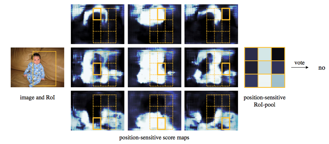
Figure 4: Visualization when an RoI does not correctly overlap the object.
R-FCN以位置敏感的RoI池化层结束。该层聚合最后一个卷积层的输出,并为每个RoI生成分数。与[8,6]不同的是,我们的位置敏感RoI层进行选择性池化,并且$k\times k$个组块中的每一个仅聚合$k\times k$分数图中一个得分图的响应。通过端到端的训练,这个RoI层可以管理最后一个卷积层来学习专门的位置敏感分数图。图1说明了这个想法。图3和图4显示了一个例子。详细介绍如下。
图3:行人类别的R-FCN(k×k=3×3)可视化。
图4:当RoI不能正确重叠目标时的可视化。
Backbone architecture. The incarnation of R-FCN in this paper is based on ResNet-101 [9], though other networks [10, 23] are applicable. ResNet-101 has 100 convolutional layers followed by global average pooling and a 1000-class fc layer. We remove the average pooling layer and the fc layer and only use the convolutional layers to compute feature maps. We use the ResNet-101 released by the authors of [9], pre-trained on ImageNet [20]. The last convolutional block in ResNet-101 is 2048-d, and we attach a randomly initialized 1024-d 1×1 convolutional layer for reducing dimension (to be precise, this increases the depth in Table 1 by 1). Then we apply the $k^2(C + 1)$-channel convolutional layer to generate score maps, as introduced next.
主干架构。本文中典型的R-FCN是基于ResNet-101[9]的,但其他网络[10,23]也适用。ResNet-101有100个卷积层,后面是全局平均池化和1000类的全连接层。我们删除了平均池化层和全连接层,只使用卷积层来计算特征映射。我们使用由[9]的作者发布的ResNet-101,在ImageNet[20]上预训练。ResNet-101中的最后一个卷积块是2048维,我们附加一个随机初始化的1024维的1×1卷积层来降维(准确地说,这增加了表1中的深度)。然后,我们应用$k^2(C+1)$通道卷积层来生成分数图,如下所述。
Position-sensitive score maps & Position-sensitive RoI pooling. To explicitly encode position information into each RoI, we divide each RoI rectangle into $k \times k$ bins by a regular grid. For an RoI rectangle of a size $w \times h$, a bin is of a size $\approx \frac{w}{k} \times \frac{h}{k}$ [8, 6]. In our method, the last convolutional layer is constructed to produce $k^2$ score maps for each category. Inside the $(i,j)$-th bin ($0 \leq i,j \leq k-1$), we define a position-sensitive RoI pooling operation that pools only over the $(i,j)$-th score map: $$r_c(i,j ~|~ \Theta) = \sum_{(x,y)\in \text{bin}(i,j)} z_{i,j,c}(x+x_0, y+y_0 ~|~ \Theta)/n. $$ Here $r_c(i,j)$ is the pooled response in the $(i,j)$-th bin for the $c$-th category, $z_{i,j,c}$ is one score map out of the $k^2(C+1)$ score maps, $(x_0, y_0)$ denotes the top-left corner of an RoI, $n$ is the number of pixels in the bin, and $\Theta$ denotes all learnable parameters of the network. The $(i,j)$-th bin spans $\lfloor i\frac{w}{k} \rfloor \leq x < \lceil (i+1)\frac{w}{k} \rceil$ and $\lfloor j\frac{h}{k} \rfloor \leq y < \lceil (j+1)\frac{h}{k} \rceil$. The operation of Eqn.(1) is illustrated in Figure 1, where a color represents a pair of $(i,j)$. Eqn.(1) performs average pooling (as we use throughout this paper), but max pooling can be conducted as well.
位置敏感的分数图和位置敏感的RoI池化。为了将位置信息显式地编码到每个RoI中,我们用规则网格将每个RoI矩形分成$k \times k$的组块。对于大小为$w \times h$的RoI矩形,组块的大小为$\approx \frac{w}{k} \times \frac{h}{k}$[8,6]。在我们的方法中,构建最后的卷积层为每个类别产生$k^2$分数图。在第$(i,j)$个组块($0 \leq i,j \leq k-1$)中,我们定义了一个位置敏感的RoI池化操作,它只在第$(i,j)$个分数映射中进行池化:$$r_c(i,j ~|~ \Theta) = \sum_{(x,y)\in \text{bin}(i,j)} z_{i,j,c}(x+x_0, y+y_0 ~|~ \Theta)/n. $$ 其中$r_c(i,j)$是第$(i,j)$个组块中第$c$个类别的池化响应,$z_{i,j,c}$是$k^2(C+1)$分数图中的一个分数图,$(x_0, y_0)$表示一个RoI的左上角,$n$是组块中的像素数量,$\Theta$表示网络的所有可学习参数。第$(i,j)$个组块跨越$\lfloor i\frac{w}{k} \rfloor \leq x < \lceil (i+1)\frac{w}{k} \rceil$和$\lfloor j\frac{h}{k} \rfloor \leq y < \lceil (j+1)\frac{h}{k} \rceil$。公式(1)的操作如图1所示,其中颜色表示一对$(i,j)$。方程(1)执行平均池化(正如我们在本文中使用的那样),但是也可以执行最大池化。
The $k^2$ position-sensitive scores then vote on the RoI. In this paper we simply vote by averaging the scores, producing a $(C+1)$-dimensional vector for each RoI: $r_c(\Theta)=\sum_{i,j}r_c(i,j ~|~ \Theta)$. Then we compute the softmax responses across categories: $s_c(\Theta)=e^{r_c(\Theta)} / \sum_{c’=0}^C e^{r_{c’}(\Theta)}$. They are used for evaluating the cross-entropy loss during training and for ranking the RoIs during inference.
$k^2$位置敏感的分数会在RoI上投票。在本文中,我们通过对分数进行平均来简单地投票,为每个RoI产生一个$(C+1)$维向量:$r_c(\Theta)=\sum_{i,j}r_c(i,j ~|~ \Theta)$。然后,我们计算跨类别的softmax响应:$s_c(\Theta)=e^{r_c(\Theta)} / \sum_{c’=0}^C e^{r_{c’}(\Theta)}$。它们被用来评估训练期间的交叉熵损失以及在推断期间的RoI名。
We further address bounding box regression [7, 6] in a similar way. Aside from the above $k^2(C+1)$-d convolutional layer, we append a sibling $4 k^2$-d convolutional layer for bounding box regression. The position-sensitive RoI pooling is performed on this bank of $4k^2$ maps, producing a $4k^2$-d vector for each RoI. Then it is aggregated into a $4$-d vector by average voting. This $4$-d vector parameterizes a bounding box as $t=(t_x, t_y, t_w, t_h)$ following the parameterization in [6]. We note that we perform class-agnostic bounding box regression for simplicity, but the class-specific counterpart (i.e., with a $4 k^2 C$-d output layer) is applicable.
我们以类似的方式进一步解决边界框回归[7,6]。除了上面的$k^2(C+1)$维卷积层,我们在边界框回归上附加了一个$4k^2$维兄弟卷积层。在这组$4k^2$维映射上执行位置敏感的RoI池化,为每个RoI生成一个$4k^2$维的向量。然后通过平均投票聚合到$4$维向量中。这个$4$维向量将边界框参数化为$t=(t_x, t_y, t_w, t_h)$,参见[6]中的参数化。我们注意到为简单起见,我们执行类别不可知的边界框回归,但类别特定的对应部分(即,具有$4k^2C$维输出层)是适用的。
The concept of position-sensitive score maps is partially inspired by [3] that develops FCNs for instance-level semantic segmentation. We further introduce the position-sensitive RoI pooling layer that shepherds learning of the score maps for object detection. There is no learnable layer after the RoI layer, enabling nearly cost-free region-wise computation and speeding up both training and inference.
位置敏感分数图的概念部分受到了[3]的启发,它开发了用于实例级语义分割的FCN。我们进一步介绍了位置敏感的RoI池化层,它可以让学习的分数图用于目标检测。RoI层之后没有可学习的层,使得区域计算几乎是零成本的,并加速训练和推断。
Training. With pre-computed region proposals, it is easy to end-to-end train the R-FCN architecture. Following [6], our loss function defined on each RoI is the summation of the cross-entropy loss and the box regression loss: $L(s, t_{x,y,w,h}) = L_{cls}(s_{c^{*}}) + \lambda [c^{*}>0] L_{reg}(t, t^*)$. Here $c^{*}$ is the RoI’s ground-truth label ($c^{*}=0$ means background). $L_{cls}(s_{c^{*}})=-\log(s_{c^{*}})$ is the cross-entropy loss for classification, $L_{reg}$ is the bounding box regression loss as defined in [6], and $t^*$ represents the ground truth box. $[c^{*}>0]$ is an indicator which equals to 1 if the argument is true and 0 otherwise. We set the balance weight $\lambda=1$ as in [6]. We define positive examples as the RoIs that have intersection-over-union (IoU) overlap with a ground-truth box of at least 0.5, and negative otherwise.
训练。通过预先计算的区域提议,很容易端到端训练R-FCN架构。根据[6],我们定义的损失函数是每个RoI的交叉熵损失和边界框回归损失的总和:$L(s, t_{x,y,w,h}) = L_{cls}(s_{c^{*}}) + \lambda [c^{*}>0] L_{reg}(t, t^*)$。这里$c^{*}$是RoI的真实标签($c^{*}=0$表示背景)。$L_{cls}(s_{c^{*}})=-\log(s_{c^{*}})$是分类的交叉熵损失,$L_{reg}$是[6]中定义的边界框回归损失,$t^*$表示真实的边界框。$[c^{*}>0]$是一个指标,如果参数为true,则等于1,否则为0。我们将平衡权重设置为$\lambda=1$,如[6]中所示。我们将正样本定义为与真实边界框重叠的交并比(IoU)至少为0.5的ROI,否则为负样本。
It is easy for our method to adopt online hard example mining (OHEM) [22] during training. Our negligible per-RoI computation enables nearly cost-free example mining. Assuming $N$ proposals per image, in the forward pass, we evaluate the loss of all $N$ proposals. Then we sort all RoIs (positive and negative) by loss and select $B$ RoIs that have the highest loss. Backpropagation [11] is performed based on the selected examples. Because our per-RoI computation is negligible, the forward time is nearly not affected by $N$, in contrast to OHEM Fast R-CNN in [22] that may double training time. We provide comprehensive timing statistics in Table 3 in the next section.
我们的方法很容易在训练期间采用在线难例挖掘(OHEM)[22]。我们可忽略的每个RoI计算使得几乎零成本的样例挖掘成为可能。假设每张图像有$N$个提议,在前向传播中,我们评估所有$N$个提议的损失。然后,我们按损失对所有的RoI(正例和负例)进行分类,并选择具有最高损失的$B$个RoI。反向传播[11]是基于选定的样例进行的。由于我们每个RoI的计算可以忽略不计,所以前向传播时间几乎不受$N$的影响,与[22]中的OHEM Fast R-CNN相比,这可能使训练时间加倍。我们在下一节的表3中提供全面的时间统计。
We use a weight decay of 0.0005 and a momentum of 0.9. By default we use single-scale training: images are resized such that the scale (shorter side of image) is 600 pixels [6, 18]. Each GPU holds 1 image and selects $B=128$ RoIs for backprop. We train the model with 8 GPUs (so the effective mini-batch size is $8\times$). We fine-tune R-FCN using a learning rate of 0.001 for 20k mini-batches and 0.0001 for 10k mini-batches on VOC. To have R-FCN share features with RPN (Figure 2), we adopt the 4-step alternating training in [18], alternating between training RPN and training R-FCN.
我们使用0.0005的权重衰减和0.9的动量。默认情况下,我们使用单尺度训练:调整图像的大小,使得尺度(图像的较短边)为600像素[6,18]。每个GPU拥有1张图像,并为反向传播选择$B=128$个RoI。我们用8个GPU来训练模型(所以有效的最小批数据大小是$8\times$)。在VOC上我们对R-FCN进行微调,使用0.001学习率进行2万次迭代和使用0.0001学习率进行1万次迭代。为了使R-FCN与RPN共享特征(图2),我们采用[18]中的四步交替训练,交替训练RPN和R-FCN。
Inference. As illustrated in Figure 2, the feature maps shared between RPN and R-FCN are computed (on an image with a single scale of 600). Then the RPN part proposes RoIs, on which the R-FCN part evaluates category-wise scores and regresses bounding boxes. During inference we evaluate 300 RoIs as in [18] for fair comparisons. The results are post-processed by non-maximum suppression (NMS) using a threshold of 0.3 IoU [7], as standard practice.
推断。如图2所示,在RPN和R-FCN之间计算共享的特征映射(在一个单一尺度的图像上)。然后,RPN部分提出RoI,R-FCN部分在其上评估类别分数并回归边界框。在推断过程中,我们评估了300个RoI进行公平比较,如[18]中那样。作为标准实践,使用0.3的IoU阈值[7],通过非极大值抑制(NMS)对结果进行后处理。
Atrous and stride. Our fully convolutional architecture enjoys the benefits of the network modifications that are widely used by FCNs for semantic segmentation [15, 2]. Particularly, we reduce ResNet-101’s effective stride from 32 pixels to 16 pixels, increasing the score map resolution. All layers before and on the conv$4$ stage 9 are unchanged; the stride=2 operations in the first conv$5$ block is modified to have stride=1, and all convolutional filters on the conv$5$ stage are modified by the “hole algorithm” [15, 2] (“Algorithme atrous”[16]) to compensate for the reduced stride. For fair comparisons, the RPN is computed on top of the conv$4$ stage (that are shared with R-FCN), as is the case in [9] with Faster R-CNN, so the RPN is not affected by the atrous trick. The following table shows the ablation results of R-FCN ($k\times k = 7\times 7$, no hard example mining). The atrous trick improves mAP by 2.6 points.

空洞和步长。我们的全卷积架构享有FCN广泛使用的语义分割的网络修改的好处[15,2]。特别的是,我们将ResNet-101的有效步长从32像素降低到了16像素,增加了分数图的分辨率。conv$4$阶段[9](stride = 16)之前和之后的所有层都保持不变;第一个conv$5$块中的stride=2操作被修改为stride=1,并且conv$5$阶段的所有卷积滤波器都被“hole algorithm”[15,2](“Algorithm atrous”[16])修改来弥补减少的步幅。为了进行公平的比较,RPN是在conv$4$阶段(与R-FCN共享)之上计算的,就像[9]中Faster R-CNN的情况那样,所以RPN不会受空洞行为的影响。下表显示了R-FCN的消融结果($k\times k = 7\times 7$,没有难例挖掘)。这个空洞窍门提高了2.6点的mAP。
Visualization. In Figure 3 and 4 we visualize the position-sensitive score maps learned by R-FCN when $k × k = 3 × 3$. These specialized maps are expected to be strongly activated at a specific relative position of an object. For example, the “top-center-sensitive” score map exhibits high scores roughly near the top-center position of an object. If a candidate box precisely overlaps with a true object (Figure 3), most of the $k^2$ bins in the RoI are strongly activated, and their voting leads to a high score. On the contrary, if a candidate box does not correctly overlaps with a true object (Figure 4), some of the $k^2$ bins in the RoI are not activated, and the voting score is low.
可视化。在图3和图4中,当$k × k = 3 × 3$时,我们可视化R-FCN学习的位置敏感分数图。期望这些专门的分数图将在目标特定的相对位置被强烈激活。例如,“顶部中心敏感”分数图大致在目标的顶部中心位置附近呈现高分数。如果一个候选框与一个真实目标精确重叠(图3),则RoI中的大部分$k^2$组块都被强烈地激活,并且他们的投票导致高分。相反,如果一个候选框与一个真实的目标没有正确的重叠(图4),那么RoI中的一些$k^2$组块没有被激活,投票分数也很低。
3. Related Work
R-CNN [7] has demonstrated the effectiveness of using region proposals [27, 28] with deep networks. R-CNN evaluates convolutional networks on cropped and warped regions, and computation is not shared among regions (Table 1). SPPnet [8], Fast R-CNN [6], and Faster R-CNN [18] are “semi-convolutional”, in which a convolutional subnetwork performs shared computation on the entire image and another subnetwork evaluates individual regions.
3. 相关工作
R-CNN[7]已经证明了在深度网络中使用区域提议[27,28]的有效性。R-CNN评估裁剪区域和变形区域的卷积网络,计算不在区域之间共享(表1)。SPPnet[8]Fast R-CNN[6]和Faster R-CNN[18]是“半卷积”的,卷积子网络在整张图像上进行共享计算,另一个子网络评估单个区域。
There have been object detectors that can be thought of as “fully convolutional” models. OverFeat [21] detects objects by sliding multi-scale windows on the shared convolutional feature maps; similarly, in Fast R-CNN [6] and [12], sliding windows that replace region proposals are investigated. In these cases, one can recast a sliding window of a single scale as a single convolutional layer. The RPN component in Faster R-CNN [18] is a fully convolutional detector that predicts bounding boxes with respect to reference boxes (anchors) of multiple sizes. The original RPN is class-agnostic in [18], but its class-specific counterpart is applicable (see also [14]) as we evaluate in the following.
有可以被认为是“全卷积”模型的目标检测器。OverFeat[21]通过在共享卷积特征映射上滑动多尺度窗口来检测目标;同样地,在Fast R-CNN[6]和[12]中,研究了用滑动窗口替代区域提议。在这些情况下,可以将一个单尺度的滑动窗口重新设计为单个卷积层。Faster R-CNN [18]中的RPN组件是一个全卷积检测器,它可以相对于多个尺寸的参考框(锚点)预测边界框。最初的RPN在[18]中是类不可知的,但是它的类特定的对应部分也是适用的(参见[14]),我们在下面进行评估。
Another family of object detectors resort to fully-connected (fc) layers for generating holistic object detection results on an entire image, such as [25, 4, 17].
另一个目标检测器家族采用全连接(fc)层来在整张图像上生成整体的目标检测结果,如[25,4,17]。
4. Experiments
###4.1 Experiments on PASCAL VOC
We perform experiments on PASCAL VOC [5] that has 20 object categories. We train the models on the union set of VOC 2007 trainval and VOC 2012 trainval (“07+12”) following [6], and evaluate on VOC 2007 test set. Object detection accuracy is measured by mean Average Precision (mAP).
4. 实验
###4.1 PASCAL VOC上的实验
我们在有20个目标类别的PASCAL VOC[5]上进行实验。我们根据[6]对VOC 2007 trainval和VOC 2012 trainval(“07 + 12”)的联合数据集进行训练,并在VOC 2007测试集上进行评估。目标检测精度通过平均精度均值(mAP)来度量。
Comparisons with Other Fully Convolutional Strategies
Though fully convolutional detectors are available, experiments show that it is nontrivial for them to achieve good accuracy. We investigate the following fully convolutional strategies (or “almost” fully convolutional strategies that have only one classifier fc layer per RoI), using ResNet-101:
与其它全卷积策略的比较
虽然全卷积检测器是可用的,但是实验表明,它们要达到良好的精度是复杂的。我们使用ResNet-101研究以下全卷积策略(或“几乎”全卷积策略,每个RoI只有一个分类器全连接层):
Naïve Faster R-CNN. As discussed in the introduction, one may use all convolutional layers in ResNet-101 to compute the shared feature maps, and adopt RoI pooling after the last convolutional layer (after conv5). An inexpensive 21-class fc layer is evaluated on each RoI (so this variant is “almost” fully convolutional). The àtrous trick is used for fair comparisons.
Naïve Faster R-CNN。如介绍中所讨论的,可以使用ResNet-101中的所有卷积层来计算共享特征映射,并且在最后的卷积层(conv5之后)之后采用RoI池化。在每个RoI上评估一个廉价的21类全连接层(所以这个变体是“几乎”全卷积的)。空洞窍门是用来进行公平比较的。
Class-specific RPN. This RPN is trained following [18], except that the 2-class (object or not) convolutional classifier layer is replaced with a 21-class convolutional classifier layer. For fair comparisons, for this class-specific RPN we use ResNet-101’s conv5 layers with the àtrous trick.
类别特定的RPN。这个RPN按照[18]进行训练,除了两类(是目标或不是)卷积分类器层被替换为21类卷积分类器层。为了公平的比较,对于这个类别特定的RPN,我们使用具有空洞窍门的ResNet-101的conv5层来处理。
R-FCN without position-sensitivity. By setting $k = 1$ we remove the position-sensitivity of the R-FCN. This is equivalent to global pooling within each RoI.
没有位置灵敏度的R-FCN。通过设置$k=1$,我们移除了R-FCN的位置灵敏度。这相当于在每个RoI内进行全局池化。
Analysis. Table 2 shows the results. We note that the standard (not naïve) Faster R-CNN in the ResNet paper [9] achieves $76.4\%$ mAP with ResNet-101 (see also Table 3), which inserts the RoI pooling layer between conv4 and conv5 [9]. As a comparison, the naïve Faster R-CNN (that applies RoI pooling after conv5) has a drastically lower mAP of $68.9\%$ (Table 2). This comparison empirically justifies the importance of respecting spatial information by inserting RoI pooling between layers for the Faster R-CNN system. Similar observations are reported in [19].
Table 2: Comparisons among fully convolutional (or “almost” fully convolutional) strategies using ResNet-101. All competitors in this table use the àtrous trick. Hard example mining is not conducted.
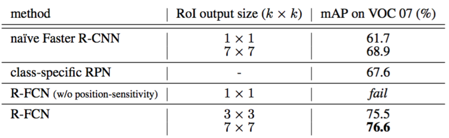
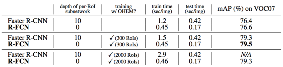
Table 3: Comparisons between Faster R-CNN and R-FCN using ResNet-101. Timing is evaluated on a single Nvidia K40 GPU. With OHEM, N RoIs per image are computed in the forward pass, and 128 samples are selected for backpropagation. 300 RoIs are used for testing following [18].
分析。表2显示了结果。我们注意到在ResNet论文[9]中的标准(非简单)Faster R-CNN与ResNet-101(参见表3)达到了$76.4\%$的mAP,在conv4和conv5之间插入了RoI池化层[9]。相比之下,简单的Faster R-CNN(在conv5之后应用RoI池化)具有$68.9\%$的更低的mAP(表2)。这种比较通过在Faster R-CNN系统的层之间插入RoI池化在经验上证明了尊重空间信息的重要性。在[19]中报道了类似的观测结果。
表2:使用ResNet-101的全卷积(或“几乎”全卷积)策略之间的比较。表中的所有竞争者都使用了空洞窍门。不执行难例挖掘。
表3:使用ResNet-101比较Faster R-CNN和R-FCN。实际是在单个Nvidia K40 GPU上评估的。使用OHEM,在前向传播中计算每张图像的N个RoI,并且选择128个样本用于反向传播。在下面的[18]中使用了300个RoI进行测试。
The class-specific RPN has an mAP of $67.6\%$ (Table 2), about 9 points lower than the standard Faster R-CNN’s $76.4\%$. This comparison is in line with the observations in [6, 12] —— in fact, the class-specific RPN is similar to a special form of Fast R-CNN [6] that uses dense sliding windows as proposals, which shows inferior results as reported in [6, 12].
类别特定的RPN具有$67.6\%$(表2)的mAP,比标准Faster R-CNN的$76.4\%$低约9个百分点。这个比较符合[6,12]中的观测结果——实际上,类别特定的RPN类似于使用密集滑动窗口作为提议的一种特殊形式的Fast R-CNN[6],如[6,12]中所报道的较差结果。
On the other hand, our R-FCN system has significantly better accuracy (Table 2). Its mAP ($76.6\%$) is on par with the standard Faster R-CNN’s ($76.4
%$, Table 3). These results indicate that our position-sensitive strategy manages to encode useful spatial information for locating objects, without using any learnable layer after RoI pooling.
另一方面,我们的R-FCN系统具有更好的准确性(表2)。其mAP($76.6\%$)与标准Faster R-CNN($76.4%$,表3)相当。这些结果表明,我们的位置敏感策略设法编码有用的空间信息来定位目标,而在RoI池化之后不使用任何可学习的层。
The importance of position-sensitivity is further demonstrated by setting $k = 1$, for which R-FCN is unable to converge. In this degraded case, no spatial information can be explicitly captured within an RoI. Moreover, we report that naïve Faster R-CNN is able to converge if its RoI pooling output resolution is 1 × 1, but the mAP further drops by a large margin to $61.7\%$ (Table 2).
位置灵敏度的重要性通过设置$k=1$来进一步证明,其中R-FCN不能收敛。在这种退化的情况下,在RoI内不能显式捕获空间信息。此外,我们还报告了,如果简单Faster R-CNN的ROI池化输出分辨率为1×1,其能够收敛,但是mAP进一步下降到$61.7\%$(表2)。
Comparisons with Faster R-CNN Using ResNet-101
Next we compare with standard “Faster R-CNN + ResNet-101” [9] which is the strongest competitor and the top-performer on the PASCAL VOC, MS COCO, and ImageNet benchmarks. We use $k × k = 7 × 7$ in the following. Table 3 shows the comparisons. Faster R-CNN evaluates a 10-layer subnetwork for each region to achieve good accuracy, but R-FCN has negligible per-region cost. With 300 RoIs at test time, Faster R-CNN takes 0.42s per image, 2.5× slower than our R-FCN that takes 0.17s per image (on a K40 GPU; this number is 0.11s on a Titan X GPU). R-FCN also trains faster than Faster R-CNN. Moreover, hard example mining [22] adds no cost to R-FCN training (Table 3). It is feasible to train R-FCN when mining from 2000 RoIs, in which case Faster R-CNN is 6× slower (2.9s vs. 0.46s). But experiments show that mining from a larger set of candidates (e.g., 2000) has no benefit (Table 3). So we use 300 RoIs for both training and inference in other parts of this paper.
与使用ResNet-101的Faster R-CNN的比较
接下来,我们与标准的“Faster R-CNN + ResNet-101”[9]进行比较,它是PASCAL VOC,MS COCO和ImageNet基准测试中最强劲的竞争对手和最佳表现者。我们在下面使用$k×k = 7×7$。表3显示了比较。Faster R-CNN评估了每个区域的10层子网络以达到良好的精度,但是R-FCN每个区域的成本可以忽略不计。在测试时使用300个RoI,Faster R-CNN每张图像花费0.42s,比我们的R-FCN慢了2.5倍,R-FCN每张图像只有0.17s(在K40 GPU上,这个数字在Titan X GPU上是0.11s)。R-FCN的训练速度也快于Faster R-CNN。此外,难例挖掘[22]没有增加R-FCN的训练成本(表3)。当从2000个RoI挖掘时训练R-FCN是可行的,在这种情况下,Faster R-CNN慢了6倍(2.9s vs. 0.46s)。但是实验表明,从更大的候选集(例如2000)中进行挖掘没有好处(表3)。所以我们在本文的其他部分使用了300个RoI来进行训练和推断。
Table 4 shows more comparisons. Following the multi-scale training in [8], we resize the image in each training iteration such that the scale is randomly sampled from {400,500,600,700,800} pixels. We still test a single scale of 600 pixels, so add no test-time cost. The mAP is $80.5\%$. In addition, we train our model on the MS COCO [13] trainval set and then fine-tune it on the PASCAL VOC set. R-FCN achieves $83.6\%$ mAP (Table 4), close to the “Faster R-CNN +++” system in [9] that uses ResNet-101 as well. We note that our competitive result is obtained at a test speed of 0.17 seconds per image, 20× faster than Faster R-CNN +++ that takes 3.36 seconds as it further incorporates iterative box regression, context, and multi-scale testing [9]. These comparisons are also observed on the PASCAL VOC 2012 test set (Table 5).
Table 4: Comparisons on PASCAL VOC 2007 test set using ResNet-101. “Faster R-CNN +++” [9] uses iterative box regression, context, and multi-scale testing.
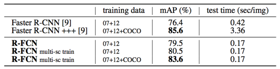
Table 5: Comparisons on PASCAL VOC 2012 test set using ResNet-101. “07++12” [6] denotes the union set of 07 trainval+test and 12 trainval. †: http://host.robots.ox.ac.uk:8080/anonymous/44L5HI.html ‡: http://host.robots.ox.ac.uk:8080/anonymous/MVCM2L.html
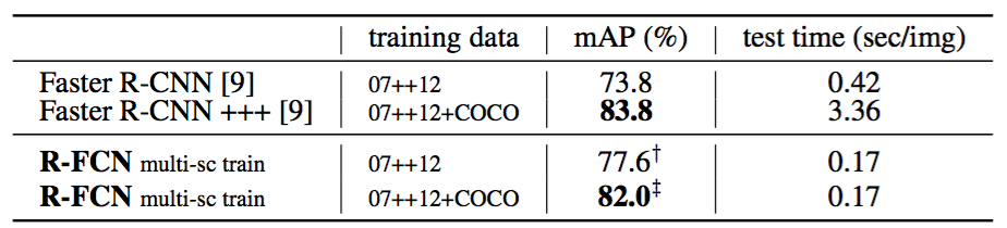
表4显示了更多的比较。在[8]中的多尺度训练之后,我们在每次训练迭代中调整图像大小,使得尺度从{400,500,600,700,800}像素中进行随机地采样。我们仍然测试600像素的单尺度,所以不添加测试时间成本。mAP是$80.5\%$。此外,我们在MS COCO [13]训练验证集上训练我们的模型,然后在PASCAL VOC数据集上对其进行微调。R-FCN达到$83.6\%$mAP(表4),接近也使用ResNet-101的[9]中的“Faster R-CNN +++”系统。我们注意到,我们的竞争结果是在每张图像0.17秒的测试速度下获得的,比花费3.36秒的Faster R-CNN +++快20倍,因为它进一步结合了迭代边界框回归,上下文和多尺度测试[9]。这些比较也可以在PASCAL VOC 2012测试集上观察到(表5)。
表4:使用ResNet-101在PASCAL VOC 2007测试集上的比较。“Faster R-CNN +++”[9]使用迭代边界框回归,上下文和多尺度测试。
表5:使用ResNet-101在PASCAL VOC 2012测试集上的比较。“07 ++ 12”[6]表示07训练+测试和12训练的联合数据集。†: http://host.robots.ox.ac.uk:8080/anonymous/44L5HI.html ‡: http://host.robots.ox.ac.uk:8080/anonymous/MVCM2L.html
On the Impact of Depth
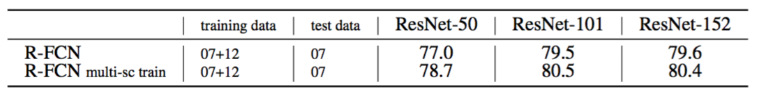
The following table shows the R-FCN results using ResNets of different depth [9]. Our detection accuracy increases when the depth is increased from 50 to 101, but gets saturated with a depth of 152.
关于深度的影响
下表显示了使用不同深度的ResNets的R-FCN结果[9]。当深度从50增加到101时,我们的检测精度增加了,但是深度达到了152。
On the Impact of Region Proposals
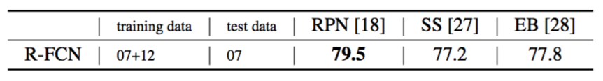
R-FCN can be easily applied with other region proposal methods, such as Selective Search (SS) [27] and Edge Boxes (EB) [28]. The following table shows the results (using ResNet-101) with different proposals. R-FCN performs competitively using SS or EB, showing the generality of our method.
关于区域提议的影响
R-FCN可以很容易地应用于其它的区域提议方法,如选择性搜索(SS)[27]和边缘框(EB)[28]。下表显示了使用不同提议的结果(使用ResNet-101)。R-FCN使用SS或EB运行,竞争性地展示了我们方法的泛化性。
4.2 Experiments on MS COCO
Next we evaluate on the MS COCO dataset [13] that has 80 object categories. Our experiments involve the 80k train set, 40k val set, and 20k test-dev set. We set the learning rate as 0.001 for 90k iterations and 0.0001 for next 30k iterations, with an effective mini-batch size of 8. We extend the alternating training [18] from 4-step to 5-step (i.e., stopping after one more RPN training step), which slightly improves accuracy on this dataset when the features are shared; we also report that 2-step training is sufficient to achieve comparably good accuracy but the features are not shared.
4.2 MS COCO上的实验
接下来,我们评估MS COCO数据集[13]中的80个目标类别。我们的实验包括8万张训练集,4万张验证集和2万张测试开发集。我们将9万次迭代的学习率设为0.001,接下来的3万次迭代的学习率设为0.0001,有效的最小批数据大小为8。我们将交替训练[18]从4步扩展到5步(即在RPN训练步骤后停止),当共享特征时略微提高了在该数据集上的准确性;我们还报告了两步训练足以达到相当好的准确性,但不共享这些特征。
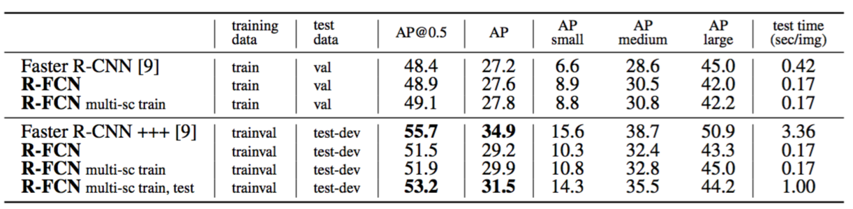
The results are in Table 6. Our single-scale trained R-FCN baseline has a val result of $48.9\%/27.6\%$. This is comparable to the Faster R-CNN baseline ($48.4\%/27.2\%$), but ours is 2.5× faster testing. It is noteworthy that our method performs better on objects of small sizes (defined by [13]). Our multi-scale trained (yet single-scale tested) R-FCN has a result of $49.1\%/27.8\%$ on the val set and $51.5\%/29.2\%$ on the test-dev set. Considering COCO’s wide range of object scales, we further evaluate a multi-scale testing variant following [9], and use testing scales of {200,400,600,800,1000}. The mAP is $53.2\%/31.5\%$. This result is close to the 1st-place result (Faster R-CNN +++ with ResNet-101, $55.7\%/34.9\%$) in the MS COCO 2015 competition. Nevertheless, our method is simpler and adds no bells and whistles such as context or iterative box regression that were used by [9], and is faster for both training and testing.
Table 6: Comparisons on MS COCO dataset using ResNet-101. The COCO-style AP is evaluated @IoU∈[0.5, 0.95]. AP@0.5 is the PASCAL-style AP evaluated @IoU=0.5.
结果如表6所示。我们单尺度训练的R-FCN基准模型的验证结果为$48.9\%/27.6\%$。这与Faster R-CNN的基准模型相当($48.4\%/27.2\%$),但我们的测试速度是Faster R-CNN的2.5倍。值得注意的是,我们的方法在小尺寸的目标上表现更好(由[13]定义)。我们的多尺度训练(但是仍是单一尺度测试)的R-FCN在验证集上的结果为$49.1\%/27.8\%$,在测试开发集上的结果是$51.5\%/29.2\%$。考虑到COCO广泛的目标尺度,按照[9]我们进一步评估多尺度的测试变种,并使用{200,400,600,800,1000}的测试尺度。mAP是$53.2\%/31.5\%$。这个结果在MS COCO 2015比赛中接近第一名的成绩(Faster R-CNN+++和ResNet-101,$55.7\%/34.9\%$)。尽管如此,我们的方法更简单,并没有添加[9]中所使用的多样功能例如上下文或迭代边界框回归,并且在训练和测试中都更快。
表6:使用ResNet-101在MS COCO数据集上比较。COCO式的AP在IoU∈[0.5,0.95]处评估。AP@0.5是PASCAL式的AP,在IoU=0.5处评估。
5. Conclusion and Future Work
We presented Region-based Fully Convolutional Networks, a simple but accurate and efficient framework for object detection. Our system naturally adopts the state-of-the-art image classification backbones, such as ResNets, that are by design fully convolutional. Our method achieves accuracy competitive with the Faster R-CNN counterpart, but is much faster during both training and inference.
5. 总结和将来的工作
我们提出了基于区域的全卷积网络,这是一个简单但精确且高效的目标检测框架。我们的系统自然地采用了设计为全卷积的最先进的图像分类骨干网络,如ResNet。我们的方法实现了与Faster R-CNN对应网络相比更具竞争力的准确性,但是在训练和推断上都快得多。
We intentionally keep the R-FCN system presented in the paper simple. There have been a series of orthogonal extensions of FCNs that were developed for semantic segmentation (e.g., see [2]), as well as extensions of region-based methods for object detection (e.g., see [9, 1, 22]). We expect our system will easily enjoy the benefits of the progress in the field.
我们故意保持R-FCN系统如论文中介绍的那样简单。已经有一系列针对语义分割(例如,参见[2])开发的FCN的正交扩展,以及用于目标检测的基于区域的方法的扩展(例如参见[9,1,22])。我们期望我们的系统能够轻松享有这个领域的进步带来的好处。
References
[1] S. Bell, C. L. Zitnick, K. Bala, and R. Girshick. Inside-outside net: Detecting objects in context with skip pooling and recurrent neural networks. In CVPR, 2016.
[2] L.-C. Chen, G. Papandreou, I. Kokkinos, K. Murphy, and A. L. Yuille. Semantic image segmentation with deep convolutional nets and fully connected crfs. In ICLR, 2015.
[3] J. Dai, K. He, Y. Li, S. Ren, and J. Sun. Instance-sensitive fully convolutional networks.arXiv:1603.08678, 2016.
[4] D. Erhan, C. Szegedy, A. Toshev, and D. Anguelov. Scalable object detection using deep neural networks. In CVPR, 2014.
[5] M. Everingham, L. Van Gool, C. K. Williams, J. Winn, and A. Zisserman. The PASCAL Visual Object Classes (VOC) Challenge. IJCV, 2010.
[6] R. Girshick. Fast R-CNN. In ICCV, 2015.
[7] R. Girshick, J. Donahue, T. Darrell, and J. Malik. Rich feature hierarchies for accurate object detection and semantic segmentation. In CVPR, 2014.
[8] K. He, X. Zhang, S. Ren, and J. Sun. Spatial pyramid pooling in deep convolutional networks for visual recognition. In ECCV. 2014.
[9] K. He, X. Zhang, S. Ren, and J. Sun. Deep residual learning for image recognition. In CVPR, 2016.
[10] A. Krizhevsky, I. Sutskever, and G. Hinton. Imagenet classification with deep convolutional neural networks. In NIPS, 2012.
[11] Y. LeCun, B. Boser, J. S. Denker, D. Henderson, R. E. Howard, W. Hubbard, and L. D. Jackel. Backpropagation applied to handwritten zip code recognition. Neural computation, 1989.
[12] K. Lenc and A. Vedaldi. R-CNN minus R. In BMVC, 2015.
[13] T.-Y. Lin, M. Maire, S. Belongie, J. Hays, P. Perona, D. Ramanan, P. Dollár, and C. L. Zitnick. Microsoft COCO: Common objects in context. In ECCV, 2014.
[14] W. Liu, D. Anguelov, D. Erhan, C. Szegedy, and S. Reed. SSD: Single shot multibox detector. arXiv:1512.02325v2, 2015.
[15] J. Long, E. Shelhamer, and T. Darrell. Fully convolutional networks for semantic segmentation. In CVPR, 2015.
[16] S. Mallat. A wavelet tour of signal processing. Academic press, 1999.
[17] J. Redmon, S. Divvala, R. Girshick, and A. Farhadi. You only look once: Unified, real-time object detection. In CVPR, 2016.
[18] S. Ren, K. He, R. Girshick, and J. Sun. Faster R-CNN: Towards real-time object detection with region proposal networks. In NIPS, 2015.
[19] S. Ren, K. He, R. Girshick, X. Zhang, and J. Sun. Object detection networks on convolutional feature maps. arXiv:1504.06066, 2015.
[20] O. Russakovsky, J. Deng, H. Su, J. Krause, S. Satheesh, S. Ma, Z. Huang, A. Karpathy, A. Khosla, M. Bernstein, A. C. Berg, and L. Fei-Fei. ImageNet Large Scale Visual Recognition Challenge. IJCV, 2015.
[21] P. Sermanet, D. Eigen, X. Zhang, M. Mathieu, R. Fergus, and Y. LeCun. Overfeat: Integrated recognition, localization and detection using convolutional networks. In ICLR, 2014.
[22] A. Shrivastava, A. Gupta, and R. Girshick. Training region-based object detectors with online hard example mining. In CVPR, 2016.
[23] K. Simonyan and A. Zisserman. Very deep convolutional networks for large-scale image recognition. In ICLR, 2015.
[24] C. Szegedy, W. Liu, Y. Jia, P. Sermanet, S. Reed, D. Anguelov, D. Erhan, and A. Rabinovich. Going deeper with convolutions. In CVPR, 2015.
[25] C. Szegedy, A. Toshev, and D. Erhan. Deep neural networks for object detection. In NIPS, 2013.
[26] C. Szegedy, V. Vanhoucke, S. Ioffe, J. Shlens, and Z. Wojna. Rethinking the inception architecture for computer vision. In CVPR, 2016.
[27] J. R. Uijlings, K. E. van de Sande, T. Gevers, and A. W. Smeulders. Selective search for object recognition. IJCV, 2013.
[28] C. L. Zitnick and P. Dollár. Edge boxes: Locating object proposals from edges. In ECCV, 2014.

